Figures

The following are some particularly useful figures in thinking about growth and development. I don’t claim that this is exhaustive, and updates may occur in the future.

The Take-off to Sustained Growth
Sustained economic growth at appreciable rates – between 0.5-2.0% per year – is a recent phenomenon. To the best of our understanding, output per capita was either stagnant at low levels or growing very slowly – like 0.05% per year – until the 19th century. At that point, growth picks up in some areas of the world and this has continued to ripple throughout the rest of the world until today. One of the most important things to note here is that the take-off to sustained economic growth in per capita output takes place at exactly the same time that population starts to grow at historically fast rates. Growth in population and growth in per capita output are not mutually exclusive, and the former probably plays a larger part in driving the latter through scale effects. My graph using data from Maddison.

Population Growth and Population Size
If population growth goes up with output per capita, and because of scale effects output per capita goes up with population size, then population growth should go up with population size. This is a really simplified intuition from Kremer (1993). And, lo and behold, this actually works in the data – this only fails in the last few decades when population growth is actually declining with population size. This is *not* because greater population is lowering output per capita, but because higher output per capita is now associated with lower population growth after the Demographic Transition. My graph using data from Kremer, updated with UN world population data for 1990’s and 2000’s.

Population and Living Standards in England
Greg Clark (2005) developed a new series on real wages for England running from the 13th century to modern day. He compared those wages to the size of the population in England at the same points in time. The figure shows that up until about 1650, there was a clear negative relationship between population and real wages – population went up, wages went down. In the 17th century this whole relationship shifts outwards, meaning that population was rising *and* wages were rising. By 1800 *both* are growing steadily over time. The breakout to sustained growth after the Industrial Revolution isn’t remarkable just because output per worker started growing, it’s remarkable because this happened despite population increasing dramatically at the same time.

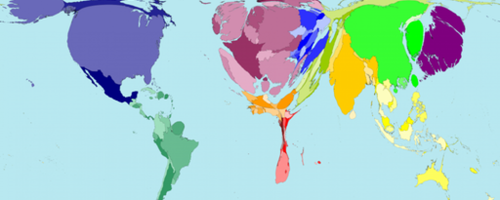
Individual Distribution of Income in 1970 and 2000
This comes from the work of Sala-i-Martin (2006), who uses country-level surveys and censuses to create the world distribution of income. The figures are density plots, which are basically histograms with really, really, narrow columns. The higher the density, the more people in the world with that income per capita. The world distribution is essentially piling the individual country distributions on top of each other, and a few of those country distributions are shown for comparison. See how the 1970 distribution is dominated by India and China, and their relative poverty. By 2000 Chinese and Indian growth has shifted the world distribution to the right.

Poverty Rates over Time
Sala-i-Martin (2006) also calculates poverty rates for several different cut-offs ($1 per day, $3 per day). You can see that at any of the levels he considers, the fraction of world population living below that level has been falling steadily over time. Because these fractions are falling faster than population is rising, the absolute number of people living below these cutoffs tends to fall over time as well.

Consistency of Growth Rates
What’s kind of remarkable about growth in developed countries is that it really seems stable, in the sense that (a) potential GDP per worker in countries grows at about 1.7-2% per year over really long periods of time and (b) that countries revert back to potential if they deviate from it. This isn’t true for all countries, just mainly the very rich countries that industrialized starting in the late 19th century and/or early 20th century. The figure shows you that there is remarkable stability in the US and UK pattern of growth (the constant slope indicates a constant growth rate, given the ratio scale of the y-axis). Germany gets dropped well below potential after WWII, but comes back rather quickly. Japan has both a dip below potential *and* a clear fundamental change in potential GDP after WWII. But note both Germany and Japan end up growing at same rate as UK and US after they reach potential.

Convergence in the OECD
Among the members of the OECD, we tend to see convergence. That is, the poorer countries are growing faster than the rich countries, implying that the poor are catching up. This suggests that the poorer countries have similar trend or potential GDP to rich countries, they just need time to reach it. Rich countries are like “adults” and poorer countries in the OECD like “kids”. Kids grow really fast because they are below their “potential” height, but eventually they’ll catch up with their parents. This convergence is consistent with a simple Solow model of growth that involves some kind of accumulated factor of production like physical capital.

Lack of Convergence in Rest of World
This convergence effect only seems to hold within the OECD. There is no tendency for *all* poor countries to grow faster than rich countries. In this figure, the poorer countries of Africa, Asia, and Latin America all fall into the bottom left, meaning they are poor and growing relatively slowly. Because they only grow as fast as rich countries, they do not catch up with rich countries over time. The big question is how come some really poor countries (e.g. Korea) make the leap to fast growth and convergence?

Conditional Convergence
Just because the poorest countries are not converging to rich country levels of output per worker doesn’t mean they are converging to something. Conditional convergence says that countries converge to their own potential level of output per worker, but that this potential differs country by country. If a country is below *its* potential, then it will tend to grow faster. This figure uses a crude estimate of a country’s potential GDP based on their characteristics in 1960 to look at conditional convergence. What you see is that countries that are farther below their potential (i.e. at 0.25 or 0.50 of their steady state) grow faster than those at their potential.

Agriculture and Non-Agriculture
This is one of my favorite figures, because there are bunch of facts that one can pull out. The output per worker in both agriculture and non-agriculture are plotted – so each country has two points in the figure. Countries that have a low share of non-agricultural workers (i.e. are heavily agricultural) have *very* low output per worker in agriculture. As countries industrialize, and the non-ag labor share rises, the agricultural output per worker is higher. The causality could run either way, but the relationship is clear. In comparison, note that non-ag output per worker is – compared to ag. output per worker – very high in countries with few non-ag workers. The variance in non-ag output per worker is very low across all countries, while the variance in ag output per worker is very high. Poor countries tend to be poor because they have (a) lots of workers in agriculture and (b) that agriculture has low output per worker.

Concentration and Diversification
Imbs and Wacziarg (2003) used industry-level data to document an really interesting pattern across countries. At low levels of GDP per capita, GDP is highly concentrated (think of everyone working in agriculture), but as GDP per capita rises concentration falls (people move out of agriculture and into a variety of other industries), and as GDP per capita gets really high concentration rises again (people end up all clustering into “Services”). This captures the general pattern of structural change well, but there is one problem with it. Most industrial classification systems were written to be very specific about manufacturing sub-industries, but lumped lots of service activities into “Services”. So it’s not clear that the rise in concentration is really reflecting a concentration of economic activity – it may just be a reflection of our classification scheme. Regardless, a neat fact to keep in mind – development is a lot about diversification.

Urbanization and Development
Urbanization is tightly linked to development. It probably is both a cause of development (allowing specialization and agglomeration) and a consequence (as people get richer they demand more “luxury” type goods that are provided in cities). People leave farms and go to live in cities. There isn’t an example of economic development in history where this *didn’t* occur. Getting rich means living in cities. However, there are some shifts over time in the exact GDP per capita/urbanization relationship. Developing countries today are more urbanized at lower levels of GDP per capita than in the past. The figure is from a working paper I have with Remi Jedwab.

Output per Worker Across Sectors
This figure is from my recent paper on the allocation of human capital across sectors. It shows the wage in a sector relative to the average wage in an economy for a sample of 14 developing countries. What you can see is that agricultural wages are almost always below the country average, while finance is almost always above. In general, people in agriculture get paid little compared to others; even if you controlled for basic human capital levels, this figure would look similar. Part of the transition to higher incomes is the shift of people out of the low wage and into the higher wage sectors. A really, really basic way to think about this shift in activity is that countries generally move left to right in this figure – from agriculture into manufacturing and then into things like services.

Savings and GDP per capita
There is a discrepancy between investment rates (investment/GDP) measured using domestic prices and measured using PPP, or world, prices. Hsieh and Klenow (2007) took a look at this. The first image is domestic-priced investment rates graphed against GPD p.c. You’ll see no big difference.

But if you look at investment and GDP valued at world prices, you get a strong positive relationship, as in the second figure. At world prices, rich countries investment more of their GDP, even though they save the same amount in domestic terms. The explanation is that investment goods are relatively expensive in poor countries. They may save 20% of their domestic income, but that just doesn’t translate into lots of investment goods. So yes, real investment is lower in poor countries, but no, that’s not necessarily because they save less.

Number of Scientists and Engineers
Maybe not too surprising, but the number of scientists and engineers has risen steadily from 1950 until today in the G-5 (US, UK, France, Germany, Japan). This fact, though, is particularly interesting from the perspective of studying growth. We think innovation is the ultimate source of economic growth, and the pure number of people working directly on what we might call “innovation” has increased dramatically, but the growth rate of GDP per capita has not changed demonstrably for about 140 years. What gives? This failure of the growth rate to change appreciably is part of why Chad Jones coined the term “semi-endogenous” growth. If the increase in the number of new ideas fails to rise linearly with the stock of ideas we already have, then the growth rate will naturally settle down to a constant rate. Even if the number of researchers jumps up, this will only have temporary effects on growth, not permanent effects. And this is what it looks like in the data.

Competition and Innovation
It probably isn’t surprising that innovation responds to the possible profits of that innovation. An important insight from endogenous growth theory – maybe the most important insight – is that these profits depend on market power, meaning a *lack* of perfect competition. Firms must be able to earn economic profits to compensate them for incurring innovation costs (under the assumption that innovation requires some resources). But if you give a firm too much market power (i.e. a pure monopoly) then it doesn’t have an incentive to innovate any more. You can see this in the data. Aghion, Bloom, Blundell, Griffith, Howitt (2005) look at businesses in the UK. When competition is low, innovation as measured by patenting is low. Innovation rises as industries get more competitive, but once you get “too much” competition, innovation falls off again. Neck-and-neck refer to industries with close competitors dominating the industry (as opposed to one major firm and lots of little competitors). (Figure is actually from Aghion et al, 2014, survey article).

Competition and Frontier Firms
A similar effect of competition shows up if we think about “frontier” firms that are highly productive already and “non-frontier” firms that are not. Increased competition for frontier firms pushes them to innovate, to maintain their market share. Increased competition for non-frontier firms pushes them to do less innovation, as they are now even less likely to be able to grab market share. Aghion, Blundell, Griffith, Howitt, and Prantl (2009) look at this with competition proxied by the entry of foreign firms in the UK. Frontier firms (those will already high productivity) see productivity grow even faster with increased competition, but non-frontier firms see productivity growth grow slowly or fall. You can think of this as explaining some of what is going on in the prior figure – when competition gets really high a lot of non-frontier firms just stop trying to innovate. (Figure is actually from Aghion et al, 2014, survey article).