Labor’s Share, Profits, and the Productivity Slowdown

NOTE: The Growth Economics Blog has moved sites. Click here to find this post at the new site.

There’s been a slowdown in measured productivity growth, particularly in the last few years, but generally since about 2000. This is something that I’ve poked around at several times, and if you’re reading economics blogs like this, then this shouldn’t be a revelation to you.

At the same time, there has been increasing attention given to the fact that labor’s share of GDP has been trending downward over the last 30 years or so. Piketty, perhaps, called the most public attention to the idea, but this is something that other people, like Loukas Karabarbounis and Brent Neiman have been working a lot on lately. The flip side of this declining labor share is a less well-documented sense that this is related to greater rents being collected by firms with more market power (Bob Solow on the topic).

What I want to do here is show how these two trends are related in some fundamental sense through how we measure productivity growth. The TL;DR version is that a falling labor share (and rising profit share of GDP) will necessarily lead to a decline in measured productivity growth, even if underlying innovation doesn’t change. The reason is that if firms have increasing market power, then they are using inputs less efficiently from an aggregate perspective, and measured productivity growth is about how efficiently we use inputs. So increased market power – captured by the decline in labor share – will put a drag on productivity growth.

Lots of math follows. None of it is too daunting, but it did end up pretty dense. When we want to measure productivity, we use a residual, because productivty cannot be directly observed. Call this measured residual productivity term
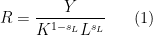
 {R}. You calculate it as

\displaystyle  R = \frac{Y}{K^{1-s_L}L^{s_L}} \ \ \ \ \ (1)

where {Y} is GDP, {K} is the capital stock, and {L} is the labor supply (which you could measure in units of human capital if you wanted). The term {s_L} is labor’s measured share in total output.

GDP is assumed to be produced according to a Cobb-Douglas function like
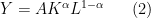
\displaystyle  Y = A K^{\alpha} L^{1-\alpha} \ \ \ \ \ (2)

where {A} is “true” productivity, which is what we are trying to get a measure of. The really important thing to note here is that {K} and {L} are raised to powers that depend on {\alpha}, not {s_L}.

{\alpha} and {1-\alpha} are “true” technological coefficients. The measure how GDP responds to stocks of capital and labor. But we don’t know them. All we know is {s_L}, labor’s share in GDP. We don’t even know capital’s share in GDP, all we know is that {1-s_L} is the left-over amount of GDP paid out as returns to capital and profits.

This wouldn’t be an issue if somehow {s_L = 1-\alpha}. And under a very precise set of conditions, these two things would be equal. If we had competition in output markets, and competition in factor markets, then {s_L = 1-\alpha}. But what are the chances that this describes the real world?

We can make a little headway if we allow for market power. The following relationship is something you can get by simply assuming that firms are cost-minimizers

\displaystyle  s_L = \frac{1-\alpha}{\mu} \ \ \ \ \ (3)

where {\mu} is the mark-up of price over its marginal cost. For example, if {\mu = 2}, then the price charged is twice the marginal cost of production (which is the cost of hiring labor and capital). Under competition, P=MC, so {\mu=1}, and {s_L = 1-\alpha}. But again, do we think we really have true competition at work in the economy? Probably not. So {\mu>1} to some extent.

Now that we know a little about {s_L}, go back to the residual calculation

\displaystyle  R = \frac{Y}{K^{1-s_L}L^{s_L}} = \frac{A K^{\alpha} L^{1-\alpha}}{K^{1-s_L}L^{s_L}} = A\left(\frac{K}{N}\right)^{s_L(1-\mu)}. \ \ \ \ \ (4)

The residual measure of productivity captures not only {A} – true productivity – but also this adjustment for the capital/labor ratio. So {R} is not a clean measure of {A} if {\mu >1}.

What is the growth rate of the residual measure of productivity? That is

\displaystyle  \frac{\dot{R}}{R} = \frac{\dot{A}}{A} - s_L(\mu-1)\frac{\dot{k}}{k} \ \ \ \ \ (5)

where I used {\dot{k}/k} as the growth rate of the capital/labor ratio, {K/N}. Again, if we had perfect competition and {\mu=1}, then the growth rate of the measured residual, {\dot{R}/R}, would be exactly equal to the growth rate of “true” productivity, {\dot{A}/A}. But once {\mu>1}, this is no longer the case, and what we can measure ({\dot{R}/R}) need not equal what we want to measure ({\dot{A}/A}).

This is a general issue. But it may not be totally deadly, because perhaps at least changes in {\dot{R}/R} could tell us about changes in {\dot{A}/A}. For example, let’s say that {s_L} and {\mu} are constant over time. And assume that the economy is essentially at steady state, so that {\dot{k}/k} is growing at the same rate as true productivity. Then if the growth rate of true productivity went down, {\dot{R}/R} would fall as well. Working that logic backwards, if the economy is at steady state and {s_L} and {\mu} are constant, then changes in the growth rate of {R} are informative about changes in the growth rate of {A}. The slowdown in measured productivity growth we see in the data would tell us that true productivity growth (innovation?) is also slowing down.

But, this isn’t true if {s_L} and {\mu} are changing. Are they changing? The labor share {s_L} is certainly falling over the last two to three decades. What about the markup, {\mu}? Is that changing?

It’s hard to measure that directly, but I think there is a way to infer that it almost certainly has been rising. Remember that relationship of {s_L = (1-\alpha)/\mu}? That came from assuming that firms are cost-minimizing (not necessarily profit-maximizing even, just cost-minimizing). That cost-minimization problem also implies that the following has to be true

\displaystyle  \text{Returns to scale} = \mu (1-s_{\pi}). \ \ \ \ \ (6)

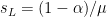
“Returns to scale” captures the returns to scale of the true production function. What I wrote above has constant returns to scale ({\alpha} plus {1-\alpha} add up to 1), and so the returns to scale are equal to 1. We can have a long argument about whether that is correct or not, but it isn’t actually crucial for the point I’m making here.

{s_{\pi}} is the share of GDP that gets paid out as profits – A/K/A rents. What this relationship says is that if the share of output going to rents rises, then so must the markup. Or think about it the other way. If firms can charge higher markups, they must be earning more in rents/profits. This is just a mechanical relationship, so it doesn’t necessarily have to be driven by one or the other.

Let’s put this all together. We’ve had a decline in the labor share of GDP, {s_L}, over the last few decades. By necessity, this implies that the share of GDP going to rents or payments to capital have risen. If the share of GDP going to rents, {s_{\pi}}, went up at all, then the markup being charged by firms, {\mu}, must have risen as well.

Let’s throw some numbers at this. Assume that {\dot{k}/k = 0.015} over the last 30 years. Let the true growth rate of innovation be {\dot{A}/A = 0.02} over the entire last 30 years (yes, an assumption). Start out 30 years ago by assuming the labor share is {s_L = 0.65} and that the markup is {\mu=1.1}, so firms charge 10% over marginal cost. This means that measured productivity growth is

\displaystyle  \frac{\dot{R}}{R} = 0.02 - 0.65\times(1.1-1)\times0.015 = 0.018 \ \ \ \ \ (7)

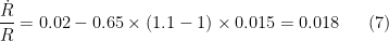
or about 1.8% per year. This is pretty close to what you see in the data for the period from 1948-1973.

Now, let the labor share fall to {s_L = 0.60}, and let the markup rise to {\mu = 1.5}. This is a pretty big markup, but for the moment I’m just trying to establish a point, so bear with me. We get that measured productivity growth is

\displaystyle  \frac{\dot{R}}{R} = 0.02 - 0.6\times(1.5-1)\times0.015 = 0.015 \ \ \ \ \ (8)

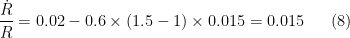
or only about 1.5% per year. Measured productivity growth has fallen, even though the underlying true productivity growth rate did not change at all.

The point is that lower measured productivity growth – {\dot{R}/R} – does not necessarily mean that actual innovation has slowed down. The decline in labor share is consistent with a rise in markups (and profit’s share of output), which will produce a drag on measured productivity growth, {\dot{R}/R}. I don’t think this story explains all of why measured productivity growth has fallen recently, but it probably plays a part.

Measured productivity growth is about how efficiently we use our inputs, and that is only partially related to the true rate of innovation. Measured productivity growth also depends on market power, because that also dictates how efficiently we use our inputs. If firms are gaining market power – meaning they can charge a higher markup – then this implies that they will use inputs less efficiently from a social perspective. Each individual firm is producing less than the amount they would under competition (with costs = marginal costs), and so we are not getting everything we can out of our inputs. If market power has increased, this exacerbates that issue, and so measured productivity – the efficiency of input use – will fall.

You cannot look at measured productivity growth, {\dot{R}/R}, and make any definitive conclusions about what is happening to true innovation or productivity growth. You cannot infer that recent innovations are less useful or productive than those that came before just because {\dot{R}/R} is falling. It may be that the policies and norms transfering some share of GDP from labor to profits/rents are pushing down the growth rate of measured productivity as well.

It’s also quite possible that you could actively work to curtail the profit share of GDP – through taxes or regulation or whatever – and yet see measured productivity rise as the markup goes down. Think about the example above, and how measured productivity growth is higher even though the markup (and hence the profit share) is lower.

Or think about the opposite situation, where you propose a policy that actively favors the profit share (lower taxes on businesses or entrepreneurs, weaker labor laws, allowing concentration of industries). It isn’t even theoretically true that this will necessarily lead to higher measured productivity growth. In the example above, any policy that tried to use lower labor shares and higher markups would have to raise the underlying growth rate of innovation by 15% – from 2% to 2.3% per year – just to break even. That is a massive change, and I think it is fair to be completely skeptical that any of those policies could raise underlying rates of innovation by that much.

There is not an either/or choice between rapid productivity growth and a higher labor share. Repeat after me: there is not an either/or choice between rapid productivity growth and a higher labor share.

A last point is that we do care explicitly about measured productivity growth if we care at all about GDP. Measured productivity growth tells us how efficiently we use inputs to produce GDP, so anything that makes measured productivity go up – better technology ({A}) or lower markups – is good for us in terms of producing GDP.

Constant versus Balanced Growth

NOTE: The Growth Economics Blog has moved sites. Click here to find this post at the new site.

Every theory of economic growth that I can think of is written to deliver “balanced growth” in the long run. Balanced growth means not only that the growth rate is constant as time goes off to infinity, but also that control variables (the savings rates, the fraction of labor allocated to R&D, the fraction of spending on education) are constant as well as time goes off to infinity.

Growth theories work hard to achieve this balanced growth, often making assumptions about functional forms to ensure that the model delivers balanced growth. Why?

The reasoning is that this is what we see in the data. Output per worker grows at roughly a constant rate in, at least, the major Western economies. If you’ve read this blog, you’ve seen a figure like this, which shows the constant growth rate over long periods of time for several economies.

But notice that all this figure indicates is that the growth rate has been constant for a Long Time. But a Long Time is not infinity, and constant growth of GDP per capita does not necessarily imply that we have a situation of balanced growth.

Just because growth is constant, this doesn’t mean that the control variables underlying growth are also constant, as is necessary for balanced growth. It is possible that we have achieved constant growth because of a fortuitous coincidence of control variables growing at rates that just offset each other such that output per person grows at a constant rate.

Chad Jones, and in a recent update Jones and Fernald, have explored whether in fact we should think of growth (in the US) as balanced growth or just as constant growth. What Jones originally suggested, and Jones and Fernald reassert, is that the control variables underlying growth in the US are not constant. Hence, the experience of the US up through 2015 may not represent balanced growth. And this in turn implies that we cannot necessarily expect the US to continue to follow the same constant growth rate in the future.

Jones and Fernald break down the roughly 2% growth in output per capita in the U.S. from 1950 to 2007 as follows:

  • 0 percentage points due to capital deepening. In short, the capital/output ratio in the US has remained roughly constant.
  • 0.4 percentage points due to increasing human capital. This is calculated from the fact that average years or schooling were rising in this period.
  • 0.4 percentage points due to scale effects. This captures the fact that increasing population generates more people doing R&D as well as larger markets that increase incentives to do R&D.
  • 1.2 percentage points due to increasing R&D intensity, meaning that the share of the labor force engaged in R&D was growing.

Of these, the increase in human capital and the increase in R&D intensity both reflect growth in control variables. In short, neither can grow forever, as they are bounded. Years of schooling is bounded by life-span (and actively removes labor from production) and the share of workers engaged in R&D cannot go above 1. So by necessity, both of those terms cannot continue to grow forever, and hence growth would have to fall below 2% as some point.

We can already see in the data that average years of education is starting to level off at about 14. And so that 0.4 p.p. we got from growing human capital may begin to disappear in the near future.

The percent of workers doing R&D has been generating much of the growth we saw over the last 50-60 years, according to Jones and Fernald. Can this continue? As I said, not forever, as that share is bounded above by 1. But we have to be careful here, as this is not just the share of workers in the US doing R&D, but something like a weighted average of the share of workers doing R&D across all countries. As China and India ramp up their shares, this can continue to pump up R&D intensity for potentially a long time. There is no obvious leveling off of R&D share, as there is with education. So perhaps we can continue on this constant (but not balanced) growth path for decades or a century longer?

Of all the terms above, only the scale effect is not a control variable, and hence is capable of continuing to provide growth forever. This means that the underlying balanced growth rate of the economy may be as low as 0.4% per year. But even that may be an overestimate, as population growth is slowing down over time.

Are we doomed to eventually see the growth rate slow down to 0.4% per year or less? Possibly. But underlying this all is a very distinct assumption about how technology evolves. Jones and Fernald, as well as nearly all growth models, assume that the flow of technology rises as technology accumulates, but at a decreasing rate. This reflects the concept that it is harder to invent new things as the number of technologies increases. By itself this would imply that the growth rate goes to zero, and it is only offset by the growth in the absolute number of R&D workers. If we stop jacking up the share of workers doing R&D, and the population size levels off, then we will no longer be able to offset this tendency for the growth rate of technology to fall towards zero.

But what if the flow of technology doesn’t have this tendency to decrease with the level of technology? We make that assumption because it delivers balanced growth in our models, but that doesn’t mean it is true. What if AI, or robots, or quantum computing, or BIG DATA, or the singularity, or aliens, or something else means that if we hit a certain level of technology, the flow of new technologies explodes? Then even with a constant number of R&D workers (or perhaps even a declining number) we could see technological growth rise and economic growth with it.

The question of what happens to growth over the next few decades boils down to two sub-questions. (A) Will the intensity of R&D effort level off, or will rich countries as well as India and China continue to push greater proportions of their resources and people into R&D? If so, then growth can be kept close to 2% for a long time. (B) Will there be a fundamental shift in the nature of technological progress?

A little aside from this discussion is that it isn’t exactly clear why we work so hard to make sure our growth models produce balanced growth, when we don’t necessarily see balanced growth in the data. Maybe its okay if your growth model has a very long-run prediction that growth is zero. We might just be on the transition path towards that zero growth rate, but it takes a very long time to get there. In the meantime, your model could be a good indicator of what is going on.