Has the Long-run Growth Rate Changed?

NOTE: The Growth Economics Blog has moved sites. Click here to find this post at the new site.

My actual job bothered to intrude on my life over the last week, so I’ve got a bit of material stored up for the blog. Today, I’m going to hit on a definitional issue that creates lots of problems in talking about growth. I see it all the time in my undergraduate course, and it is my fault for not being clearer.

If I ask you “Has the long-run growth rate of the U.S. declined?”, the answer depends crucially on what I mean by “long-run growth rate”. I think of there as being two distinct definitions.

  • The measured growth rate of GDP over a long period of time: The measured long-run growth rate of GDP from 1985 to 2015 is {(\ln{Y}_{2015} - \ln{Y}_{1985})/30}. Note that here the measurement does not have to take place using only past data. We could calculate the expected measured growth rate of GDP from 2015 to 2035 as {(\ln{Y}_{2035} - \ln{Y}_{2015})/20}. Measured growth rate depends on the actual path (or expected actual path) of GDP.
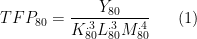
  • The underlying trend growth of potential GDP: This is the sum of the trend growth rate of potential output per worker (we typically call this {g}) and the trend growth rate of the number of workers (which we’ll call {n}).

The two ways of thinking about long-run growth inform each other. If I want to calculate the measured growth rate of GDP from 2015 to 2035, then I need some way to guess what GDP in 2035 will be, and this probably depends on my estimate of the underlying trend growth rate.

On the other hand, while there are theoretical avenues to deciding on the underlying trend growth rate (through {g}, {n}, or both), we often look back at the measured growth rate over long periods of time to help us figure trend growth (particularly for {g}).

Despite that, telling me that one of the definitions of the long-run growth rate has fallen does not necessarily inform me about the other. Let’s take the work of Robert Gordon as an example. It is about the underlying trend growth rate. Gordon argues that {n} is going to fall in the next few decades as the US economy ages and hence the growth in number of workers will slow. He also argues that {g} will fall due to us running out of useful things to innovate on. (I find the argument regarding {n} strong and the argument regarding {g} completely unpersuasive. But read the paper, your mileage may vary.)

Now, is Gordon right? Data on the measured long-run growth rate of GDP does not tell me. It is entirely possible that relatively slow measured growth from around 2000 to 2015 reflects some kind of extended cyclical downturn but that {g} and {n} remain just where they were in the 1990s. I’ve talked about this before, but statistically speaking it will be decades before we can even hope to fail to reject Gordon’s hypothesis using measured long-run growth rates.

This brings me back to some current research that I posted about recently. Juan Antolin-Diaz, Thomas Drechsel, and Ivan Petrella have a recent paper that finds “a significant decline in long-run output growth in the United States”. [My interpretation of their results was not quite right in that post. The authors e-mailed with me and cleared things up. Let’s see if I can get things straight here.] Their paper is about the measured growth rate of long-run GDP. They don’t do anything as crude as I suggested above, but after controlling for the common factors in other economic data series with GDP (etc.. etc..) they find that the long-run measured growth rate of GDP has declined over time from 2000 to 2014. Around 2011 they find that the long-run measured growth rate is so low that they can reject that this is just a statistical anomaly driven by business cycle effects.

What does this mean? It means that growth has been particularly low so far in the 21st century. So, yes, the “long-run measured growth rate of GDP has declined” in the U.S., according to the available evidence.

The fact that Antolin-Diaz, Drechsel, and Petrella find a lower measured growth rate similar to the CBO’s projected growth rate of GDP over the next decade does not tell us that {g} or {n} (or both) are lower. It tells us that it is possible to reverse engineer the CBO’s assumptions about {g} and {n} using existing data.

But this does not necessarily mean that the underlying trend growth rate of GDP has actually changed. If you want to establish that {g} or {n} changed, then there is no retrospective GDP data that can prove your point. Fundamentally, predictions about {g} and {n} are guesses. Perhaps educated guesses, but guesses.

Significant Changes in GDP Growth

NOTE: The Growth Economics Blog has moved sites. Click here to find this post at the new site.

A relatively quick post to highlight two other posts that recently came out regarding GDP growth. First, David Papell and Ruxandra Prodan have a guest post up at Econbrowser regarding the long-run effects of the Great Recession. They use the CBO projections of GDP into the future (similar to what I did here) and look at whether there was a statistically significant break in the level of GDP at the Great Recession. Short answer, yes. Their testing finds that the break was 2008:Q2, not a surprising date to end up with.

It is important to remember that David and Ruxandra are testing for a break in the level of GDP, and not GDP per capita. It is entirely possible to have a structural break in GDP while not having a structural break in GDP per capita. The next thing to remember is that they cannot reject that the growth rate of GDP is the same after 2008:Q2 as it was before. What I mean is easier to see in their figure than it is to explain:
Papell Prodan
Before and after the break, the growth rate is identical. It is just the level that has changed.

The second post is from Juan Antolin-Diaz, Thomas Drechsel, and Ivan Petrella. They use only existing data (not CBO projections) and find that there is statistical evidence of a change in the growth rate of U.S. GDP. They see a slowdown in growth starting in the mid-2000’s, consistent with John Fernald’s suggestions regarding productivity growth. It takes until 2015 to see this break statistically because you need several years of data to confirm that the growth slowdown was not a temporary phenomenon.

Note the subtle but very, very, very important difference between the two posts. Papell/Prodan find a significant shift in the level of GDP, while Antolin-Diaz, Drechsel, and Petrella (ADP) find a significant shift in the growth rate of GDP. The former sucks, but the latter is far more troubling. If the growth rate is truly lower, then we will get farther and farther away from the pre-GR trend, and the ratio of actual GDP to pre-GR trend GDP will go to zero. If it is just a level shift, then the ratio of actual GDP to pre-GR trend GDP will go to one as both become arbitrarily large.

I find the Papell/Prodan result more convincing. Keep in mind that David is my department chair and if I knocked on my office wall right now I could interrupt the phone call he is on. Ruxandra’s office is all of 20 feet from mine. I see these people every day. But regardless of the fact that I know them personally, I think they are right.

ADP are getting a false result showing slow growth because of the level shift that David and Ruxandra identify. If ADP do not allow for the level shift, then over any window of time that includes 2008:Q2 the growth rate will be calculated to be low. But that is just a statistical artifact of this one-time drop in GDP. It doesn’t mean that the long-run growth rate is in fact different. Put it this way: if they re-run their tests 25 years from now, they’ll find no statistical evidence of a growth change.

Of course, if the CBO is wrong about the path of GDP from 2015-2025, then Papell/Prodan could be wrong and ADP could be right. But given the current CBO projections, there is strong evidence of a negative level shift to GDP, but no change in the long-run growth rate.

Is the U.S. Really Below Potential GDP?

NOTE: The Growth Economics Blog has moved sites. Click here to find this post at the new site.

The CBO just released a new projection of both GDP and the budget out to 2024. In short, the CBO sees the U.S. staying below potential GDP for several years. Menzie Chinn just did a short review of how people use inflation and/or unemployment to try and figure out the difference difference between actual and potential GDP.

From a growth perspective, I wanted to take a look at the projections a little differently. First, I don’t much care about the level of aggregate GDP, I care about the level of GDP per capita. So I took the CBO numbers and combined them with population figures and projections to get actual and projected GDP per capita for the U.S. Note, I’m using the CBO projections for actual GDP, not their potential GDP numbers. I want to look at the expected GDP numbers.

Second, I wanted to consider how this projected GDP per capita compared to long-run trends, rather than using inflation or unemployment to assess whether GDP per capita is “at potential”. I am looking instead whether GDP per capita has deviated from its long-run path. To do this I merged the GDP per capita projections from the CBO with the Maddison dataset on GDP per capita from 1970 to 2008. (The CBO goes back far enough that the two series overlap and I can adjust the actual levels of GDP per capita to match).

I took the trend in GDP per capita from 1990 to 2007, and extrapolated that out from 2008 to 2024. Then I plotted the actual and CBO-projected GDP per capita data against that trend. Here is what you get:
Post 1990 Trend
It’s clear here that in 2007 GDP per capita drops below the 1990-2007 trend line. Moreover, the CBO expects that GDP per capita will stay below that trend line out until 2024. It looks like a distinct “level shift” in the parlance of growth economics. GDP per capita is something like 13% below the 1990-2007 trend.

If you look at the post-war trend in GDP per capita from 1947 to 2007, you get something similar. The gap in 2024, 18% below trend, is actually worse than the gap using the post-1990 era.
Post War Trend

But if you extend your view back even further, and incorporate the whole period of 1870-2007 to form the trend line, things look different. Now, if you plot the projected GDP per capita against the trend, it looks as if the U.S. is spot on.
All Data Trend
GDP per capita is almost exactly where you’d expect it given the historical trend. The CBO expects GDP per capita to be a little low in 2024, about 2% behind the full trend line. Using the 1870-2007 trend, there doesn’t appear to be anything particularly unusual about the projected path of GDP per capita. The U.S. seems to be moving along the same balanced growth path it always has.

What really looks like the anomaly in U.S. data is the extended period from about 1990 to 2010 that we spent above trend. You could think of this as capturing John Fernald’s argument (or see here) that the IT boom of the 1990’s was a one-time level shift up in GDP. We got a big boost from that, but now the economy is settling back to the long-run growth path.

[You should not – NOT – use this as an argument that the financial crash and subsequent recession were necessary, useful, or welfare-improving. It is quite possible for the economy to have managed a graceful slide back to the long-run trend line after 2007 rather than experiencing it all in one dramatic plunge. The long-run trend is like gravity. Yes, it will win in the end, but that does not mean that I have to leap to the ground after cleaning out my gutters. I have a ladder.]

I really thought when I started playing with this data that I’d be writing a post about how the Great Recession had fundamentally shifted GDP per capita below the long-run trend, and that this represented a really fundamental shock given how stable the long-run trend had been until now. But the current path of GDP per capita doesn’t appear to be that surprising in historical perspective.

The big caveat here is that the CBO could be entirely wrong about future GDP per capita growth. If they have been overly optimistic, then we could certainly find ourselves falling below even the very long-run trend. Then again, they could have been pessimistic, and we might find ourselves above trend for all I know. But even with all the uncertainty, the expectation is that the U.S. economy will find itself right where you would have predicted it would be.

Techno-neutrality

NOTE: The Growth Economics Blog has moved sites. Click here to find this post at the new site.

I’ve had a few posts in the past few months (here and here) about the consequences of mechanization for the future of work. In short, what will we do when the robots take our jobs?

I wouldn’t call myself a techno-optimist. I don’t think the arrival of robots necessarily makes everything better. But I do not buy the strong techno-pessimism that comes up in many places. Richard Serlin has been a frequent commenter on this blog, and he generally has a gloomy take on where we are going to end up once the robots arrive. I’m not bringing up Richard to pick on him. He writes thoughtful comments on this subject (and lots of others), and it is those comments that pushed me to try and be more clear on why I’m “techno-neutral”.

The economy is more creative than we can imagine. The coming of robots to mechanize away our jobs is the latest in a long, long, long, history of technology replacing workers. And yet here we still are, working away. Timothy Taylor posted this great selection a few weeks ago. This is a quote from Time Magazine:

The rise in unemployment has raised some new alarms around an old scare word: automation. How much has the rapid spread of technological change contributed to the current high of 5,400,000 out of work? … While no one has yet sorted out the jobs lost because of the overall drop in business from those lost through automation and other technological changes, many a labor expert tends to put much of the blame on automation. … Dr. Russell Ackoff, a Case Institute expert on business problems, feels that automation is reaching into so many fields so fast that it has become “the nation’s second most important problem.” (First: peace.)
The number of jobs lost to more efficient machines is only part of the problem. What worries many job experts more is that automation may prevent the economy from creating enough new jobs. … Throughout industry, the trend has been to bigger production with a smaller work force. … Many of the losses in factory jobs have been countered by an increase in the service industries or in office jobs. But automation is beginning to move in and eliminate office jobs too. … In the past, new industries hired far more people than those they put out of business. But this is not true of many of today’s new industries. … Today’s new industries have comparatively few jobs for the unskilled or semiskilled, just the class of workers whose jobs are being eliminated by automation.

That quote is from 1961. This is almost word for word the argument you will get about robots and automation leading to mass unemployment in the future. 50 years ago we were just as worried about this kind of thing, and in those 50 years we do not have massive armies of unemployed workers wandering the streets. The employment/population ratio in 1961 was about 55%, and then it steadily rose until the late 90’s when it topped out at about 64%. Even after the Great Recession, the ratio is still 59% today, higher than it was in 1961.

This didn’t happen without disruption and dislocation. And the robots will cause similar dislocation and disruption. Luddites weren’t wrong about losing their jobs, they were just wrong about the economy losing jobs in aggregate. But I don’t see why next-generation robots are any different than industrial robots, mainframes, PC’s, tractors, mechanical looms, or any other of the ten million innovations made in history that replaced labor. We can handle this with some sympathy and try to smooth things out for those dislocated, or we can do what usually happens and let them hang out to dry. The robots aren’t the problem here, we are.

What exactly are those new jobs that will be created? If I knew, then I wouldn’t be writing this blog post, I’d be out starting a company. The fact that I cannot conceive of an innovation myself is not evidence that innovation has ceased. But I do believe in the law of large numbers, and somewhere among the 300-odd million Americans is someone who *is* thinking of a new kind of company with new kinds of jobs.

Robots change prices as well as wages. An argument for pessimism goes like this. People have subsistence requirements, meaning they have a wage floor below which they cannot survive. Robots will be able to replace humans in production and this will drive the wage below that subsistence requirement. Either no firm will hire workers at the subsistence wage or people who do work will not meet subsistence.

The problem with this argument is that it ignores the impact of robots on the price of that subsistence requirement. Subsistence requirements are in real terms (I need clothes and housing and food), not nominal terms (I need $2000 dollars). The “subsistence wage” is a a real wage, meaning it is the nominal wage divided by the price level of a subsistence basket of goods. Robots lowering marginal costs of production lowers the nominal human wage, but it also lowers the price of goods. It is not necessary or even obvious that real wages have to fall because of robots. History says that despite all of the labor-saving technological change that has gone on over the last few hundred years, real wages have risen as the lower costs outweigh the downward pressure on wages.

Who is going to buy what the robots produce? Call this the “Henry Ford” argument. If you are going to invest in opening up a factory staffed entirely by robots, then who precisely is supposed to buy that output? Ford raised wages at his highly mechanized (for the time) plants so that he had a ready-made market for his cars. The Henry Fords of robot factories are going to need a market for the stuff they build. Rich people are great, but diminishing marginal utility sets in pretty quick. That means robot owners either need to lower prices or raise wages for the people they do hire in order to generate a big enough market. Depending on the fixed costs involved in getting these proverbial robot factories up and running, robot owners may be a strong force for keeping wages high in the economy, just like Henry Ford was back in the day.

The wealthy are wealthy because they own productive assets. A tiny fraction of the value of those assets is due to the utility to the owner of the widgets they kick out. The majority of the value of those assets is due to the fact that you can *sell* that output for money and use that money to buy other widgets. Rockefeller wasn’t wealthy because he had a lot of oil. He was wealthy because he could sell it to other people. No other people, no wealth. Just barrel after barrel of useless black gunk.

The same holds for robot owners. Those robots and robot factories have value because you can sell them or the goods they make in the wider economy. And that means continuing to exchange with the non-wealthy. You cannot be wealthy in a vacuum. Bill Gates on an island with robots and a stack of 16 billion dollar bills is Gilligan with a lot of kindling.

Wealthy robot owners will do what wealthy (fill in capital stock here) owners have done for eons. They’ll trade access to the capital, or the goods it produces, to the non-wealthy in exchange for services, effort, flattery, and new ideas on what to do with that wealth.

Wealth concentration would be a problem with or without robots. The worry here is that because the wealthy will be the only ones able to build the robots and robot factories, they will control completely the production of goods and the demand for labor. That’s not a problem that arises with robots, that is a problem that arises with, well, settled agriculture 10,000 years ago. Wealth concentration makes owners both monopolists (market power selling goods) and monopsonists (market power buying labor), which is a bad combination. It gives them the ability to drive (real) wages down to minimum subsistence levels. This is bad, absolutely. But this was bad when (fill in example of a landed elite) did it in (fill in historical era here). This is bad in “company towns”. This is bad now, today. So if you want to argue against wealth concentration and the pernicious influence it has on wages, get started. Don’t wait for the robots, they’ve got nothing to do with it.

Again, be clear that in arguing against techno-pessimism I am not arguing that robots will generate a techno-utopia with ponies and rainbows. I just do not buy the dystopian view that somehow it’s all going to come crashing down around our ears because of the very particular innovations coming in the near future.

Why Did Consumption TFP Stagnate?

NOTE: The Growth Economics Blog has moved sites. Click here to find this post at the new site.

I’ve been trying to think more about why consumption-sector TFP flatlined from about 1980 forward. What I mentioned in the last post about this was that the fact that TFP was constant does not imply that technology was constant.

I then speculated that technology in the service sector may not have changed much over the last 30 years, partly explaining the lack of consumption productivity growth. By a lack of change, I mean that the service sector has not found a way to produce more services for a given supply of inputs, and/or produced the same amount of service with a decreasing supply of inputs. Take something that is close to a pure service – a back massage. A one-hour back massage in 1980 is almost identical to a one-hour back massage in 2014. You don’t get twice (or any other multiple) of the massage in 2014 that you got in 1980. And even if the therapist was capable of reducing back tension in 30 minutes rather than 60, you bought a 60-minute massage.

We often buy time when we buy services, not things. And it isn’t so much time as it is attention. And it is very hard to innovate such that you can provide the same amount of attention with fewer inputs (i.e. workers). Because for many services you very specifically want the attention of a specific person for a specific amount of time (the massage). You’d complain to the manager if the therapist tried to massage someone else at the same appointment.

So we don’t have to be surprised that even technology in services may not rise much over 30 years. But there were obviously technological changes in the service sector. As several people brought up to me, inventory management and logistics were dramatically changed by IT. This allows a service firm to operate “leaner”, with a smaller stock of inventory.

But this kind of technological progress need not show up as “technological change” in doing productivity accounting. That is, what we call “technology” when we do productivity accounting is not the only kind of technology there is. The “technology” in productivity accounting is only the ability to produce more goods using the same inputs, and/or produce the same goods using fewer inputs. It doesn’t capture things like a change in the shape of the production function itself, say a shift to using fewer intermediate goods as part of production.

Let’s say a firm has a production function of {Y = AK^{\alpha}L^{\beta}M^{\gamma}} where {A} is technology in the productivity sense, {K} is capital, {L} is labor, and {M} is intermediate goods. Productivity accounting could reveal to us a change in {A}. But what if an innovation in inventory management/logistics means that {\gamma} changes?

If innovation changes the shape of the production function, rather than the level, then our TFP calculations could go anywhere. Here’s an example. Let’s say that in 1980 production is {Y_80 = A_{1980}K_{80}^{.3}L_{80}^{.3}M_{80}^{.4}}. Innovation in logistics and inventory management makes the production function in 2014
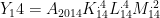
 {Y_14 = A_{2014}K_{14}^{.4}L_{14}^{.4}M_{14}^{.2}}.

Total factor productivity in 1980 is calculated as

\displaystyle  TFP_{80} = \frac{Y_{80}}{K_{80}^{.3}L_{80}^{.3}M_{80}^{.4}} \ \ \ \ \ (1)

and total factor productivity in 2014 is calculated as

\displaystyle  TFP_{14} = \frac{Y_{14}}{K_{14}^{.4}L_{14}^{.4}M_{14}^{.2}}. \ \ \ \ \ (2)

TFP in 2014 relative to 1980 (the growth in TFP) is

\displaystyle  \frac{TFP_{14}}{TFP_{80}} = \frac{Y_{14}}{K_{14}^{.3}L_{14}^{.3}M_{14}^{.4}} \times \frac{K_{80}^{.3}L_{80}^{.3}M_{80}^{.4}}{Y_{80}} \times \frac{M_{14}^{.2}}{K_{14}^{.1}L_{14}^{.1}} \ \ \ \ \ (3)

which is an unholy mess. The first fraction is TFP in 2014 calculated using the 1980 function. The second fraction is the reciprocal of TFP in 1980, calculated normally. So the first two fractions capture the relative TFP in 2014 to 1980, holding constant the 1980 production function. The last fraction represents the adjustment we have to make because the production function changed.

That last term could literally be anything. Less than one, more than one, more than 100, less than 0.0001. If {K} and {L} rose by a lot while {M} didn’t go up much, this will lower TFP in 2014 relative to 1980. It all depends on the actual units used. If I decide to measure {M} in thousands of units rather than hundreds of units, I just made TFP in 2014 go down by a factor of 4 relative to 1980.

Once the production function changes shape, then comparing TFP levels across time becomes nearly impossible. So in that sense TFP could definitely be “getting it wrong” when measuring service-sector productivity. You’ve got an apples to oranges problem. So if we think that IT innovation really changed the nature of the service-sector production function – meaning that {\alpha}, {\beta}, and/or {\gamma} changed, then TFP isn’t necessarily going to be able to pick that up. It could well be that this looks like flat or even shrinking TFP in the data.

If you’d like, this supports David Beckworth‘s notion that consumption TFP “doesn’t pass the smell test”. We’ve got this intuition that the service sector has changed appreciably over the last 30 years, but it doesn’t show up in the TFP measurements. That could be due to this apples to oranges issue, and in fact consumption TFP doesn’t reflect accurately the innovations that occurred.

To an ambitious graduate student: document changes in the revenue shares of intermediates in consumption and/or services over time. Correct TFP calculations for these changes, or at least provide some notion of the size of that fudge factor in the above equation.

The Limited Effect of Reforms on Growth

NOTE: The Growth Economics Blog has moved sites. Click here to find this post at the new site.

I said in my last post that transitional growth is slow, and therefore changing potential GDP – as many of the recent Cato Growth proposals would do – could not add much to the growth rate of GDP in the near term.

There were several questions that came up in the comments, so let me try to be more clear about distinguishing between influences of trend growth and short-run shocks. Output in period {t+1} is

\displaystyle  y_{t+1} = (1+g)y_t + (1+g)\lambda (y^{\ast}_t - y_t) \ \ \ \ \ (1)

where the first term on the right is the normal trend growth rate, and the second term is the additional transitional growth that occurs because the economy is not at potential GDP, {y^{\ast}_t}.

We need to distinguish between changes in potential GDP and changes in current GDP. Let’s take the above equation, plug in {\lambda=0.02}, and then use it to iterate forward from period 0 (today) until some arbitrary period {t}. You get

\displaystyle  y_t = (1+g)^t \left[(1-0.98^t)y^{\ast}_0 + 0.98^t y_0 \right]. \ \ \ \ \ (2)

In period {t}, GDP will have grown by a factor of {(1+g)^t} due to trend growth in GDP. The term in the brackets shows the cumulative effect of having {y_0 \neq y^{\ast}_0} in the initial period. The 0.98 terms are just {1-.02}, and capture the changing role of this transitional growth over time. Note that as {t} goes up, {0.98^t} goes to zero and the effect of initial GDP {y_0} falls to nothing. As {t} gets big, the economy reaches potential GDP.

Now let’s assume that period 0 is 2014. Potential GDP is 17 trillion and actual GDP is 16 trillion, and the trend growth rate is 2%. Let’s consider two alternative policies to enact today that take effect in 2015.

  • Policy A: a short run spending surge sufficient to make GDP in 2015 equal to potential GDP. Policy A immediately eliminates the gap between actual and potential GDP, but has no other long term effect.
  • Policy B: raises potential GDP by 1 trillion dollars, but adds no immediate spending to GDP. The effect on potential GDP is permanent.

For Policy A, GDP in 2015 (period 1) is

\displaystyle  y_1 = (1.02)^1\left[(1-0.98)\times 17 + 0.98 \times 17 \right] = 17.34. \ \ \ \ \ (3)

The growth rate of GDP from 2014 to 2015 is {(17.34 - 16)/16 = 0.084} or about 8.4%. That’s a massive GDP growth rate for a developed economy like the US. But it is a one-time shock to the growth rate. From 2015 to 2016, and from 2016-2017, and every year thereafter, the growth rate will be exactly 2% because the economy is precisely back on trend. Policy A gives a one-year gigantic boost to the growth rate.

What about Policy B? GDP in 2015 here is

\displaystyle  y_1 = (1.02)^1\left[(1-0.98)\times 18 + 0.98 \times 16 \right] = 16.36. \ \ \ \ \ (4)

This is nearly 1 trillion less than Policy A. The growth rate of GDP from 2014 to 2015 is {(16.36 - 16)/16 = 0.023}. As the prior post noted, reforms that raise potential GDP don’t have big effects on growth rates. But while the effect on growth is small, it is persistent. From 2015-2016, the growth rate of GDP will be roughly…0.023. It’s actually minutely smaller than from 2014-2015, but rounding makes them look the same. It will take a few years before the growth rate declines appreciably. Fifty years from now the growth rate will still be almost 0.021. Changing potential GDP, like with Policy B, is like turning an oil tanker with a tug boat. It doesn’t go fast, but it goes on for a long time.

So is Policy B worse than Policy A? It depends entirely on your time preferences. In 2015 GDP under Policy A is nearly 1 trillion dollars higher than with policy B. But 100 years from now, GDP will be nearly 1 trillion dollars higher with Policy B. We can actually figure out how soon it will be before Policy B passes Policy A. Set

\displaystyle  (1.02)^t \left[(1-0.98^t)17 + 0.98^t 17 \right] = (1.02)^t \left[(1-0.98^t)18 + 0.98^t 16 \right] \ \ \ \ \ (5)

and solve for {t}. This turns out to be roughly 34 years from now, in 2048. It takes a long, long, time for changes in potential GDP to really pay off. If you want to increase the level of GDP in the near term, and hence raise near-term growth rates by implication, then you have to, you know, boost GDP. GDP is a measure of current spending, so raising GDP means raising current spending. There isn’t a trick to get around this.

Now, could I be underselling Policy B as a near-term boost to growth rates and GDP? Let’s consider a few possibilities:

  • I’m underestimating the size of {\lambda}. As I mentioned last time, there is lots of empirical evidence that this is pretty small. But okay, let’s make {\lambda = 0.05}, more than double my 0.02 value. Now in 2015 policy B yields GDP of 16.4 trillion and a growth rate of 2.6%. Yes, it helps policy B, but doesn’t get it anywhere close to Policy A. It is still 14 years before GDP under Policy B is larger than under Policy A.
  • I’m underestimating the boost to potential GDP that Policy B can deliver. So let’s ask, given {\lambda = 0.05}, how much would {y^{\ast}_0} have to go up to match the 8.4% growth rate of Policy A? Potential GDP would have to jump to roughly 36 trillion, meaning it has to roughly **double** in size thanks to the policy. I think it is totally fair to say that this is implausible in a country like the US.
  • But China was able to do it. Right, when China opened up, made reforms, etc.., it was able to raise its potential GDP by a large amount. You could probably plausibly argue that it raised potential GDP by a factor of something like 8-10. But the rapid growth in China over the last 30 years is not some victory lap for good state-led policy reforms, it’s a testament to just how screwed up Maoism was as an economic system. [Egad! An institutions explanation!]
  • What if Policy B raised the trend growth rate, {g}? If it changed {g} appreciably, then Policy B would be something really special. Let’s review for a moment a few of the changes that did not change the long-run growth rate in the US: the introduction of electricity, the income tax, the Great Depression, the New Deal, Medicare, higher tax rates, the Cold War, the oil crisis, lower tax rates, de-regulation, the IT revolution, and New Coke. There have been shifts in the level of potential GDP, such as the IT revolution shifting up potential GDP and inducing a period of relatively rapid transitional growth in the 1990’s. But it’s hard – if not impossible if you take Chad Jones‘ semi-endogenous growth idea seriously – to fundamentally alter {g}. It is dictated by changes in the scale of the global economy, not by policy effects within the US.

I’m all for policy reforms that raise potential GDP, and several of those proposed in the Cato forum would probably do that. We might want to undertake several of them at once to counteract the drags on potential GDP that Robert Gordon has outlined.

But we can’t be fooled into thinking that any of them would make a really appreciable difference to economic growth today. You can revolutionize education, or corporate taxation, or urban planning, or immigration all you want, but the gains those changes induce will take decades to manifest themselves.

[insert policy here] Won’t Boost Growth Rates

NOTE: The Growth Economics Blog has moved sites. Click here to find this post at the new site.

Over at the Cato Institute, they hosted an online forum about reviving economic growth. There are lots of smart people involved. The web page has lots of big pictures of their heads, I guess to indicate that their brains are like, totally huge.

Anyway, each one wrote up some proposed policy reform that would help boost long-run growth prospects. Brad DeLong responded to many of the proposals here before his head exploded reading Doug Holtz-Eakin’s essay.

I’m not going to quibble with any of the minutiae of the proposals. My point is going to be a general one on the possible growth effects of [insert policy here]. Short answer, there won’t be any.

There are two ways to boost GDP growth. Either

  • Actively raise current GDP through increased spending by some sector of the economy.
  • Raise potential GDP and let transitional growth speed up.

The second one perhaps deserves a little explanation. Transitional growth is an extra boost to growth that occurs when current GDP is below potential GDP. Why does this occur? Bob Solow is why. In an economy with accumulable factors of production (physical capital, human capital, knowledge capital) being below potential GDP means that the return to these factors is relatively high, and hence more investment in those factors is done, boosting GDP growth. The wider is the gap between current and potential GDP, the stronger this transitional growth.

The issue is that [insert policy here] is a policy to raise potential GDP, not current GDP. But the transitional effects this encourages are inherently small. So even if [insert policy here] opens up a big gap between potential and actual GDP, this doesn’t translate into much extra growth. In fact, the effects are likely so small that they would be unnoticeable against the general noise in growth rates year by year.

To give you an idea of how little an effect [insert policy here] will have on growth, let’s play with math. Output in period {t+1} can be written in terms of output in period {t} this way

\displaystyle  y_{t+1} = (1+g)[y_t + \lambda (y^{\ast}_t - y_t)]. \ \ \ \ \ (1)

This says that output in {t+1} is equal to {1+g} times current output. That is “regular” growth. The term with the {\lambda} is the additional boost in growth we get from being below potential. {y^{\ast}_t} is potential GDP in period {t}, and {y^{\ast}_t - y_t} is the gap in GDP. {\lambda} tells us how much of that gap we make up from period {t} to {t+1}. If {\lambda = 0}, then we are stuck below potential (secular stagnation). If {\lambda = 1}, then immediately next period our GDP will be at potential again.

Let’s think about this in terms of growth rates, so

\displaystyle  Growth = \frac{y_{t+1}-y_t}{y_t} = (1+g)\left[\lambda \frac{y^{\ast}_t}{y_t} + (1-\lambda)\right] - 1. \ \ \ \ \ (2)

The growth rate from {t} to {t+1} depends on the ratio of potential to actual GDP today, period {t}. If that ratio were equal to one – meaning that we were at potential – then the growth rate just becomes {g}, the trend growth rate. The larger is {y^{\ast}_t/y_t} – meaning the farther we are from potential – the higher is the actual growth rate.

Now we can go back to thinking about the possible growth impact of [insert policy here]. GDP today ({y_t}) is about 16 trillion. Potential GDP today ({y^{\ast}_t}) is probably about 17 trillion. You can get a lower estimate from the CBO, Robert Gordon, or John Fernald, or a higher estimate from older CBO forecasts. I’m going to err on the high side for potential because this will inflate the growth effect of [insert policy here].

We also need to know the value of {\lambda}, the percent of the GDP gap that is closed in a year. We’ve got lots of evidence that this value is about {\lambda = 0.02}, or 2% of the gap closes every year. This estimate goes back to the original cross-country convergence literature starting with Barro (1991), but consistently across samples (countries, US states, Japanese prefectures, Canadian provinces, etc..) economies converge to potential GDP at about 2% of the gap per year.

You get higher values of {\lambda} if you assume that economies pursue optimal savings plans, like in the Ramsey model, meaning that they save at a higher rate when they are farther below steady state. But if there is an economy that saves according to the predictions of the Ramsey model, it is populated by unicorns.

Back to the calculation. The last thing we need is a value for {g}, trend growth. Let’s call that {g = 0.02}, or trend growth in GDP is about 2% per year. Again, we can argue about whether that is higher or lower, but that’s not going to be the important factor here.

Okay, so based on the fact that we are currently 1 trillion below trend, the growth rate today should be

\displaystyle  Growth = (1+.02)\left[.02 \frac{17}{16} + (1-.02)\right] - 1 = .0213 \ \ \ \ \ (3)

or growth should be 2.13%. Growth will be about 0.13 percentage points higher than normal – that’s a little over one-tenth of one percent – because we are below potential. The value of {g} is really irrelevant. All the action is inside the brackets. Because {\lambda} is small, there isn’t much bite from transitional growth, even though we are $1 trillion below trend.

But what about [insert policy here]? That will *raise* potential GDP, and therefore will induce faster transitional growth to the new, higher potential GDP. Okay. Let’s say that [insert policy here] has an astonishingly positive impact on potential GDP. I mean massive. [insert policy here] adds a full $1 trillion to potential GDP, which is now $18 trillion. Now, growth under the [insert policy here] regime is

\displaystyle  Growth = (1+.02)\left[.02 \frac{18}{16} + (1-.02)\right] - 1 = .0225 \ \ \ \ \ (4)

Uh, wow? Growth will be an additional 0.12 percentage points higher thanks to [insert policy here]. This is not a massive change in growth. And the growth boost will *decline* over time as we get closer to potential.

Fine, but what if [insert policy here] is truly revolutionary, and raises potential GDP by $2 trillion? Then growth will be 0.0238. This could be generously rounded to 0.025, meaning you added a half-point to the growth rate of GDP. But let’s not kid ourselves that [insert policy here] is going to have that big of an effect on growth. $2 trillion implies that [insert policy here] is raising potential GDP by about 12%. That would be an anomaly of historic proportions.

[insert policy here] will not generate any appreciable extra economic growth, even though in the very long-run [insert policy here] may be a net positive for the level of economic activity. The problem is that it takes a very, very, very long time for those positive effects to manifest themselves, and thus [insert policy here] won’t do anything to fundamentally change GDP growth.

What about the exceptions I mentioned? Among the proposals, there are a few that could boost current GDP (and thus growth) directly and immediately by encouraging spending.

  • Scott Sumner’s NGDP targeting. The proposal speaks directly to raising current GDP, as opposed to raising potential GDP. I think of this as solving the balance sheet problems of households. Boost nominal spending and nominal incomes rise, while nominal debts like mortgages remain fixed, leading to extra spending.
  • Brad DeLong’s raising K-12 teacher salaries. If you could do it *now*, then it would raise incomes for these folks, and boost spending. The second part of the proposal, to tie this to teacher tenure changes, is more of a potential GDP changer. Question, how big of an impact would this really have on spending?
  • A number of people mention infrastructure spending. Yes, if we would spend that money *now*, then it would materially boost GDP growth *now*, and as a bonus have long-run benefits for potential GDP.

Ultimately, the issue in the U.S. right now is not with potential GDP. We do not need policies to raise this potential GDP so much as we need policies to get us back to potential. That requires actively boosting immediate spending.

Why I Care about Inequality

NOTE: The Growth Economics Blog has moved sites. Click here to find this post at the new site.

“Inequality” is a term that has been tossed about quite a bit. The Occupy movement, to Piketty’s book, to debates over the minimum wage, to Greg Mankiw‘s defense of the 1%. Just today Mark Thoma published an op-ed on inequality. A few days ago John Cochrane had a post about why we care about inequality.

One of Cochrane’s main points is that the term “inequality” has been used in so many contexts, and to refer to so many different things, that it is ceasing to lose meaning. I’ll agree with him on this completely. If you want to talk about “inequality”, you have to be very clear about what precisely you mean.

There are three things that people generally mean by “inequality”:

  1. The 1% versus the 99%. That is, the difference in average annual income of the top 1% of all households versus the average annual income of the bottom 99%.
  2. The stagnation of median real wages and those below the median.
  3. The college premium, or the gap in earnings between those who finished college and those who did not (or did not attend).

When I say I care about inequality, I mean mainly the second – the stagnation of median wages – but this is going to take me into territory covered by the first – the growth in top 1% income. There are things to say about the college premium, but I’m not going to say them here.

Why do I care about the stagnation of median wages?

  • Because I’m going to be better off if everyone shares in prosperity. I want services like education, health care, and home repairs to be readily available and cheap. The way to achieve that is to invest in developing a large pool of skilled workers – teachers, nurses, electricians, carpenters. Those at the bottom of the distribution don’t have sufficient income to make those investments privately, so that requires public provision of those investments (i.e. schools) or transfers to support private investments. You want to have an argument about whether public provision or transfers are more efficient? Okay. But the fact that there is an argument on implementation doesn’t change the fact that stagnant wages are a barrier to these investments right now.
  • Because people at the bottom of the income distribution aren’t going to disappear. We can invest in these people, or we can blow our money trying to shield ourselves from them with prisons, police officers, and just enough income support to keep them from literally starving. I vote for investment.

One response to this is that I don’t care about inequality per se, I care about certain structural issues in labor markets, education, and law enforcement. So why don’t we address those fundamental structural issues, rather than waving our hands around about inequality, which is meaningless? Because these strutural issues are a problem of under-investment. The current allocation of income/wealth across the population is not organically producing enough of this investment, so that allocation is a problem. In short, if you care about these structural issues, you cannot escape talking about the distribution of income/wealth. In particular, you have to talk about another kind of inequality, the 1%/99% kind.

Let me be very clear about this too, because I don’t want anyone to think I’m trying to be clever and hide something. I would take some of the income and/or wealth from people with lots of it, and then (a) give some of that to currently poor people so they can afford to make private investments and (b) use the rest to invest in public good provision like education, infrastructure, and health care.

Would I use a pitchfork and torches to do this? No. Would I institute “confiscatory taxation” on rich people? No, that’s a meaningless term that Cochrane and others use to suggest that somehow rich people are going to be persecuted for being rich. I am talking about raising marginal income tax rates and estate tax rates back to the archaic levels seen in the 1990s.

Why do I not feel bad about taxing rich people further?

  • Because rich people spend their money on useless stuff. Not far from where I live, there is a new house going up. It will be over 10,000 square feet when it is complete. 2,500 of those square feet will be a closet that has two separate floors, one for regular clothes and one for formal wear. If that is what you are spending your money on, then yes, I believe raising your taxes to fund education, infrastructure, and health spending is a net gain for society.

    Don’t poor people spend money on stupid stuff? Of course they do. Isn’t the government an inefficient provider of some of these goods, like education? Maybe. But even if both those things are true, public investment and/or transfers to poor people will result in some net investment that I’m not currently getting from the mega-closet family. I’m happy to talk about alternative institutional settings that would ensure a greater proportion of the funds get spent on actual investments.

  • Because I’m not afraid that some embattled, industrious core of “makers” will decide to “go Galt” and drop out of society, leaving the rest of us poor schleps to fend for ourselves. Oh, however will we figure out how to feed ourselves without hedge fund managers around to guide us?

    This is actually a potential feature of higher marginal tax rates, by the way, not a bug. You’re telling me that a top tax rate at 45% will convince a number of wealthy self-righteous blowhards (*cough* Tom Perkins *cough*) to flee the country? Great. Tell me where they live, I’ll help them pack. And even if these self-proclaimed “makers” do stop working, the economy is going to be just fine. How do I know? Imagine that the entire top 1% of the earnings distribution left the country, took all of their money with them, and isolated themselves on some Pacific island. Who’s going to starve first, them or the remaining 300-odd million of us left here? The income and wealth of the top 1% have value only because there is an economy of another 300-odd million people out there willing to provide services and make goods in exchange for some of that income and wealth.

So, yes, I care about 1%/99% inequality itself, because I cannot count on the 1% to privately make good investment decisions regarding the human capital of the bottom 99%. And the lack of investment in the human capital of the bottom part of the income distribution is a colossal waste of resources.

The Slowdown in Reallocation in the U.S.

NOTE: The Growth Economics Blog has moved sites. Click here to find this post at the new site.

One of the components of productivity growth is reallocation. From one perspective, we can think about the reallocation of homogenous factors (labor, capital) from low-productivity firms to high-productivity firms, which includes low-productivity firms going out of business, and new firms getting started. A different perspective is to look more closely at the shuffling of heterogenous workers between (relatively) homogenous firms, with the idea being that workers may be more productive in one particular environment than in another (i.e. we want people good at doctoring to be doctors, not lawyers). Regardless of how exactly we think about reallocation, the more rapidly that we can shuffle factors into more productive uses, the better for aggregate productivity, and the higher will be GDP. However, evidence suggests that both types of reallocation have slowed down recently.

Foster, Grim, and Haltiwanger have a recent NBER working paper on the “cleansing effect of recessions”. This is the idea that in recessions, businesses fail. But it’s the really crappy, low-productivity businesses that fail, so we come out of the recession with higher productivity. The authors document that in recessions prior to the Great Recession, downturns tend to be “cleansing”. Job destruction rates rise appreciably, but job creation rates remain about the same. Unemployment occurs because it takes some time for those people whose jobs were destroyed to find newly created jobs. But the reallocation implied by this churn enhances productivity – workers are leaving low productivity jobs (generally) and then getting high productivity jobs (generally).

But the Great Recession was different. In the GR, job destruction rose by a little, but much less than in prior recessions. Job creation in the GR fell demonstrably, much more than in prior recessions. So again, we have unemployment as the people who have jobs destroyed are not able to pick up newly created jobs. But because of the pattern to job creation and destruction, there is little of the positive reallocation going on. People are not losing low productivity jobs, becoming unemployed, and then getting high productivity jobs. People are staying in low productivity jobs, and new high productivity jobs are not being created. So the GR is not “cleansing”. It is, in some ways, “sullying”. The GR is pinning people into *low* productivity jobs.

This holds for firm-level reallocation well. In recessions prior to the GR, low productivity firms tended to exit, and high productivity firms tended to grow in size. So again, we had productivity-enhancing recessions. But again, the GR is different. In the GR, the rate of firm exit for low productivity firms did not go up, and the growth rate of high-productivity firms did not rise. The GR is not “cleansing” on this metric either.

Why is the GR so different? The authors don’t offer an explanation, as their paper is just about documenting these changes. Perhaps the key is that a financial crash has distinctly different effects than a normal recession. A lack of financing means that new firms cannot start, and job creation falls, leading to lower reallocation effects. A “normal” recession doesn’t involve as sharp a contraction in financing, so new firms can take advantage of others going out of business to get themselves going. Just an idea, I have no evidence to back that up.

[An aside: For the record, there is no reason that we need to have a recession for this kind of reallocation to occur. Why don’t these crappy, low-productivity firms go out of business when unemployment is low? Why doesn’t the market identify these crappy firms and compete them out of business? So don’t take Foster, Grim, and Haltiwanger’s work as some kind of evidence that we “need” recessions. What we “need” is an efficient way to reallocate factors to high productivity firms without having to make those factors idle (i.e. unemployed) for extended periods of time in between.]

In a related piece of work Davis and Haltiwanger have a new NBER working paper that discusses changes in workers reallocations over the last few decades. They look at the rate at which workers turn over between jobs, and find that in general this rate has declined since 1980 to today. Some of this may be structural, in the sense that as the age structure and education breakdown of the workforce changes, there will be changes in reallocation rates. In general, reallocation rates go down as people age. 19-24 year olds cycle between jobs way faster than 55-65 year olds. Reallocation rates are also higher among high-school graduates than among college graduates. So as the workforce has aged and gotten more educated from 1980 to today, we’d expect some decline in job reallocation rates.

But what Davis and Haltiwanger find is that even after you account for these forces, reallocation rates for workers are declining. No matter which sub-group you look at (e.g. 25-40 year old women with college degrees) you find that reallocation rates are falling over time. So workers are flipping between jobs *less* today than they did in the early 1980s. Which is probably somewhat surprising, as my guess is that most people feel like jobs are more fleeting in duration these days, due to declines in unionization, etc.. etc..

The worry that Davis and Haltiwanger raise is that lower rates of reallocation lower productivity growth, as mentioned at the beginning of this post. So what has caused this decline in reallocation rates across jobs (or across firms as the first paper described)? From a pure accounting perspective, Davis and Haltiwanger gives us several explanations. First, reallocation rates within the Retail sector have declined, and since Retail started out with one of the highest rates of reallocation, this drags down the average for the economy. Second, more workers tend to be with older firms, which have less turnover than young firms. Last, the above-mentioned shift towards an older workforce that tends to shift jobs less than younger workers.

Fine, but what is the underlying explanation? Davis and Haltiwanger offer several possibilities. One is increased occupational licensing. In the 1950s, only about 5 % of workers needed a government (state or federal) license to do their job. In 2008, that is now 29%. So it can be incredibly hard to reallocate to a new job or sector of work if you have to fulfill some kind of licensing requirement (which could involve up to 2000 hours of training along with fees). Second is a decreased ability of firms to fire-at-will. Starting in the 1980s there were a series of court decisions that made it harder for firms to just fire someone, which makes it both less likely for people to leave jobs, and less likely for firms to hire new people. Both act to lower reallocation between jobs. Third is employer-provided health insurance, which generates some kind of “job lock” where people are unwilling to move jobs because they don’t want to lose, or create a gap in, coverage.

Last is the information revolution which may have had perverse effects on reallocation. We might expect that IT allows more efficient reallocation as people can look for jobs more easily (e.g. Monster.com, LinkedIn) and firms can cast a wider net for applicants. But IT also allows firms to screen much more effectively, as they have access to credit reports, criminal records, and the like, that would have been prohibitive to acquire in the past.

So we appear to have, on two fronts, declining dynamic reallocation in the U.S. This certainly contributes to a slowdown in productivity growth, and may perhaps be a better explanation than “running out of ideas from the IT revolution” that Gordon and Fernald talk about. The big worry is that, if it is regulation-creep, as Davis and Haltiwanger suspect, we don’t know if or when the slowdown in reallocation would end.

In summary, reading John Haltiwanger papers can make you have a bad day.

Age Structure, Experience, Productivity…… and France!

NOTE: The Growth Economics Blog has moved sites. Click here to find this post at the new site.

Miles Kimball posted a link to a relatively old Scott Sumner post that was discussing a Paul Krugman post from 2011. Which means I am only about 3 years behind, which is good, because I would have estimated I was about 5 years behind.

Anyway, Scott’s post deals with some facts about France. Namely, while GDP per capita in France is only roughly 70% of the U.S. level, GDP per hour worked is essentially equal to that in the U.S. French workers are just as productive per hour as U.S. workers, but just work fewer hours in aggregate.

There are generally two responses to this. The optimistic one: “The French have made a decision to spend their high productivity by taking more vacations and retiring earlier, leading to lower GDP per capita, but probably higher utility.” The pessimistic one: “The French labor system is so mucked up by taxes and regulations that despite being as productive per hour as the U.S., firms do not find it profitable, and workers do not find it desirable, to have more hours provided.”

It’s non-obvious which view is correct. Scott’s post makes two great points, though, about how to think about this. The first is one that I’m not going to deal with here. Comparing France to the U.S. is not an apples to apples comparison. The U.S. is better compared to the EU, or at least Western Europe, as a whole. French productivity looks much worse when compared to New England or the Mid-Atlantic as a region, and only looks good in comparison to the U.S. because the U.S. includes Mississippi and Alabama (which I will arbitrarily call the Sicily and Greece of Europe). It’s a great point.

The second idea that Scott talks about is whether we should be impressed by French output per hour being as high as the U.S. In France, the high youth unemployment rate and early retirement rate mean that the employed population is concentrated in the 30-55 age range. If this age range tends to be particularly productive compared to other age groups, then shouldn’t French output per hour be much higher than in the U.S., where we employ lots of sub-30 and over-55 workers?

Jim Feyrer has a paper from a few years back that looks precisely at the relationship of age structure and measures of productivity. What he finds is that the most productive group of workers are those aged 40-49. An 1% increase in the number of those workers (holding other age groups constant) is associated with about a 0.2% increase in productivity. Ages 50-plus imply lower productivity, but the statistical significance is low. Ages under 39, though, are significantly negative for productivity. Jim uses these relationships to partly explain the productivity slowdown in the US during the 1970s, when the Baby Boomers were filling up the labor force and were still under 40, meaning they were relatively low productivity.

But the results speak to this French question that Scott poses as well. By employing so few under 39-year-olds, France is essentially only using the very high productivity workers in the economy. Thus their GDP per hour is likely inflated by that fact, and their workers are not necessarily just as productive as those in the U.S. What you’d want is some kind of equivalent measure for the U.S. to make this concrete. What is the age-structure-adjusted GDP per hour worked in the U.S. and France? Based on Jim’s results, the U.S. would be ahead in that comparison.

This is related to the well-known result in labor economics that wages rise with labor market experience, but at a decreasing rate. That is, people’s wages always tend to rise with experience, but once you hit about 25-30 years of experience (meaning you are somewhere between 40-55 most likely, the increase gets close to zero. You can see a bunch of these wage/experience relationships in a paper by Lagakos, Moll, Porzio, and Qian, who compare the relationship across countries. One of the features of the data is that in rich countries (like France and the U.S.) the wage/experience relationship is really, really steep when experience is below 10 years. In other words, wages are particularly low for people who have little labor market experience, like young workers aged 18-25.

The U.S. tends to employ a lot more 18-25 year olds as a fraction of our labor force than France. Even prior to 2007, unemployment among those under 25 was roughly 20% in France, and only 10% in the U.S., see here. So the U.S. is employing far more workers that have not yet hit the sweet spot in labor market experience and their wages are very low. On the assumption that wages are some indication of how productive workers are, this means that the U.S. employs proportionately more low-productivity workers. So, again, France’s measured GDP per hour should really be higher than the U.S. level if in fact France and the U.S. have similar productivity levels.

Scott’s point is that we can’t take the equivalence between France’s and the U.S.’s GDP per hour at face value. This doesn’t necessarily mean that the pessimistic view noted above is correct. France could well be making some kind of optimal decision to take lots of leisure time and retirement. But that decision is not one made with the same “budget constraint” as the U.S. – France is very likely not as productive as the U.S.

If you do want to subscribe to the pessimistic viewpoint, then you could argue that not only have French regulations mucked up the labor market, but they have also given the statistical illusion of high productivity. Hence, France is in fact much worse off than the U.S. Even if they fixed their labor market, their GDP per capita would not reach U.S. levels.