NOTE: The Growth Economics Blog has moved sites. Click here to find this post at the new site.
One of the most active area of research in macro development (let’s not call it growth economics, I guess) is on misallocations. This is the concept that a major explanation for why some countries are rich, while others are poor, is that rich countries do a good job of allocating factors of production in an efficient manner across firms (or sectors, if you like). Poor countries do a bad job of this, so that unproductive firms use a lot of labor and capital up, while high productivity firms are too small.
One of the baseline papers in this area is by Diego Restuccia and Richard Rogerson, who showed that you could theoretically generate big losses to aggregate measures of productivity if you introduced firm-level distortions that acted like subsidies to unproductive firms and taxes on produtive firms. This demonstrated the possible effects of misallocation. A paper by Hsieh and Klenow (HK) took this idea seriously, and applied the basic logic to data on firms from China, India and the U.S. to see how big of an effect misallocations actually have.
We just went over this paper in my grad class this week, and so I took some time to get more deeply into the paper. The one flaw in the paper, from my perspective, was that it ran backwards. That is, HK start with a detailed model of firm-level activity and then roll this up to find the aggregate implications. Except that I think you can get the intuition of their paper much more easily by thinking about how you measure the aggregate implications, and then asking yourself how you can get the requisite firm-level data to make the aggregate calculation. So let me give you my take on the HK paper, and how to understand what they are doing. If you’re seriously interested in studying growth and development, this is a paper you’ll need to think about at some point, and perhaps this will help you out.
This is dense with math and quite long. You were warned.
What do HK want to do? They want to compare the actual measured level of TFP in sector  ,
,  , to a hypothetical level of TFP in sector ,
  , that we would measure if we allocated all factors efficiently between firms.
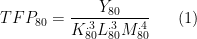
Let’s start by asking how we can measure given observable data on firms. This is
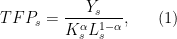
which is just measuring for a sector as a Solow residual. is not a pure measure of “technology”, it is a measure of residual productivity, capturing everything that influences how much output ( ) we can get from a given bundle of inputs (
 ). It includes not just the physical productivity of individual firms in this sector, but also the efficiency of the distribution of the factors across those firms.
Now, the issue is that we cannot measure directly. For a sector, this is some kind of measure of real output (e.g. units of goods), but there is no data on that. The data we have is on revenues of firms within the sector (e.g. dollars of goods sold). So what HK are going to do is use this revenue data, and then make some assumptions about how firms set prices to try and back out the real output measure. It’s actually easier to see in the math. First, just write as
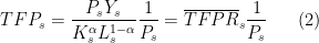
which just multiplies and divides by the price index for sector . The first fraction is revenue productivity, or  , of sector . This is a residual measure as well, but measures how produtive sector is at producing dollars, rather than at producing units of goods. The good thing about
  is that we can calculate this from the data. Take the revenues of all the firms in sector , and that is equal to total revenues
  . We can add up the reported capital stocks across all firms, and labor forces across all firms, and get
  and
and  , respectively. We can find a value for
  based on the size of wage payments relative revenues (which should be close to
  ). So all this is conceptually measurable.
The second fraction is one over the price index  . We do not have data on this price index, because we don’t know the individual prices of each firms output. So here is where the assumptions regarding firm behavior come in. HK assume a monopolistically competitive structure for firms within each sector. This means that each firm has monopoly power over producing its own brand of good, but people are willing to substitute between those different brands. As long as the brands aren’t perfectly substitutable, then each firm can charge a price a little over the marginal cost of production. We’re going to leave aside the micro-economics of that structure for the time being. For now, just trust me that if these firms are monopolistically competitive, then the price index can be written as

where  are the individual prices from each firm, and
  is the elasticity of substitution between different firms goods.
Didn’t I just say that we do not observe those individual firm prices? Yes, I did. But we don’t need to observe them. For any individual firm, we can also think of revenue productivity as opposed to their physical productivity, denoted  . That is, we can write
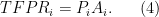
The firms productivity at producing dollars ( ) is the price they can charge () times their physical productivity (). We can re-arrange this to be

Put this expression for firm-level prices into the price index we found above. You get
![\displaystyle P_s = \left(\sum_i \left[\frac{TFPR_i}{A_i}\right]^{1-\sigma} \right)^{1/(1-\sigma)} \ \ \ \ \ (6)](https://s0.wp.com/latex.php?latex=%5Cdisplaystyle++P_s+%3D+%5Cleft%28%5Csum_i+%5Cleft%5B%5Cfrac%7BTFPR_i%7D%7BA_i%7D%5Cright%5D%5E%7B1-%5Csigma%7D+%5Cright%29%5E%7B1%2F%281-%5Csigma%29%7D+%5C+%5C+%5C+%5C+%5C+%286%29&bg=ffffff&fg=000000&s=0&c=20201002)
which depends only on firm-level measure of and physical productivity . We no longer need prices.
For the sector level , we now have
![\displaystyle TFP_s = \overline{TFPR}_s \frac{1}{P_s} = \frac{\overline{TFPR}_s}{\left(\sum_i \left[\frac{TFPR_i}{A_i}\right]^{1-\sigma} \right)^{1/(1-\sigma)}}. \ \ \ \ \ (7)](https://s0.wp.com/latex.php?latex=%5Cdisplaystyle++TFP_s+%3D+%5Coverline%7BTFPR%7D_s+%5Cfrac%7B1%7D%7BP_s%7D+%3D+%5Cfrac%7B%5Coverline%7BTFPR%7D_s%7D%7B%5Cleft%28%5Csum_i+%5Cleft%5B%5Cfrac%7BTFPR_i%7D%7BA_i%7D%5Cright%5D%5E%7B1-%5Csigma%7D+%5Cright%29%5E%7B1%2F%281-%5Csigma%29%7D%7D.+%5C+%5C+%5C+%5C+%5C+%287%29&bg=ffffff&fg=000000&s=0&c=20201002)
At this point, there is just some slog of algebra to get to the following
![\displaystyle TFP_s = \left(\sum_i \left[A_i \frac{\overline{TFPR}_s}{TFPR_i}\right]^{\sigma-1} \right)^{1/(\sigma-1)}. \ \ \ \ \ (8)](https://s0.wp.com/latex.php?latex=%5Cdisplaystyle++TFP_s+%3D+%5Cleft%28%5Csum_i+%5Cleft%5BA_i+%5Cfrac%7B%5Coverline%7BTFPR%7D_s%7D%7BTFPR_i%7D%5Cright%5D%5E%7B%5Csigma-1%7D+%5Cright%29%5E%7B1%2F%28%5Csigma-1%29%7D.+%5C+%5C+%5C+%5C+%5C+%288%29&bg=ffffff&fg=000000&s=0&c=20201002)
If you’re following along at home, just note that the exponents involving flipped sign, and that can hang you up on the algebra if you’re not careful.
Okay, so now I have this description of how to measure . I need information on four things. (1) Firm-level physical productivities, , (2) sector-level revenue productivity, , (3) firm-level revenue productivities, , and (4) a value for . Of these, we can appeal to the literature and assume a value of , say something like a value of 5, which implies goods are fairly substitutable. We can measure sector-level and firm-level revenue productivities directly from the firm-level data we have. The one big piece of information we don’t have is , the physical productivity of each firm.
Before describing how we’re going to find , just consider this measurement of for a moment. What this equation says is that is a weighted sum of the individual firm level physical productivity terms, . That makes some sense. Physical productivity of a sector must depend on the productivity of the firms in that sector.
Mechanically, is a concave function of all the stuff in the parentheses, given that  is less than one. Meaning that goes up as the values in the summation rise, but at a decreasing rate. More importantly, for what HK are doing, this implies that the greater the variation in the individual firm-level terms of the summation, the lower is . That is, you’d rather have two firms that have similar productivity levels than one firm with a really big productivity level and one firm with a really small one. Why? Because we have imperfect substitution between the output of the firms. Which means that we’d like to consume goods in somewhat rigid proportions (think Leontief perfect complements). For example, I really like to consume one pair of pants and one shirt at the same time. If the pants factory is really, really productive, then I can lots of pants for really cheap. If the shirt factory is really un-productivie, I can only get a few shirts for a high price. To consume pants/shirts in the desired 1:1 ratio I will end up having to shift factors away from the pants factor and towards the shirt factory. This lowers my sector level productivity.
There is nothing that HK can or will do about variation in across firms. That is taken as a given. Some firms are more productive than others. But what they are interested in is the variation driven by the terms. Here, we just have the extra funkiness that the summation depends on these inversely. So a firm with a really high is like having a really physically unproductive firm. Why? Think in terms of the prices that firms charge for their goods. A high means that firms are charging a relatively high price compared to the rest of the sector. Similarly, a firm with a really low (like our shirt factory above) would also be charging a relatively high price compared to the rest of the sector. So having variation in across firms is like having variation in , and this variation lowers .
However, as HK point out, if markets are operating efficiently then there should be no variation in across firms. While a high is similar to a low in its effect on , the high arises for a fundamentally different reason. The only reason a firm would have a high compared to the rest of the sector is if it faced higher input costs and/or higher taxes on revenues than other firms. In other words, firms would only be charging more than expected if they had higher costs than expected or were able to keep less of their revenue.
In the absence of different input costs and/or different taxes on revenues, then we’d expect all firms in the sector to have identical . Because if they didn’t, then firms with high could bid away factors of production from low firms. But as high firms get bigger and produce more, the price they can charge will get driven down (and vice versa for low firms), and eventually the terms should all equate.
For HK, then, the level of that you could get if all factors were allocated efficiently (meaning that firms didn’t face differential input costs or revenue taxes) is one where  for all firms. Meaning that

So what HK do is calculate both and (as above), and compare.
To do this, I already mentioned that the one piece of data we are missing is the terms. We need to know the actual physical productivity of firms. How do we get that, since we cannot measure physical output at the firm level? HK’s assumption about market structure will allow us to figure that out. So hold on to the results of and for a moment, and let’s talk about firms. For those of you comfortable with monopolistic competition models using CES aggregators, this is just textbook stuff. I’m going to present it without lots of derivations, but you can check my work if you want.
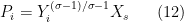
For each firm, we assume the production function is

and we’d like to back out as
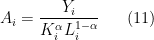
but we don’t know the value of  . So we’ll back it out from revenue data.
Given that the elasticity of substitution across firms goods is , and all firms goods are weighted the same in the utility function (or final goods production function), then the demand curve facing each firm is
where  is a demand shifter that depends on the amount of the other goods consumed/produced. We going to end up carrying this term around with us, but it’s exact derivation isn’t necessary for anything. Total revenues of the firm are just

Solve this for , leaving  together as revenues. This gives you

Plug this in our equation for to get

This last expression gives us a way to back out from observable data. We know revenues,  , capital,
  , and labor,
  . The only issue is this thing. But is identical for each firm – it’s a sector-wide demand term – so we don’t need to know it. It just scales up or down all the firms in a sector. Both and will be proportional to , so when comparing them will just cancel out. We don’t need to measure it.
What is our measure picking up? Well, under the assumption that firms in fact face a demand curve like we described, then is picking up their physical productivity. If physical ouput, , goes up then so will revenues, . But not proportionally, as with more output the firm will charge a lower price. Remember, the pants factory has to get people to buy all those extra pants, even though they kind of don’t want them because there aren’t many shirts around. So the price falls. Taking revenues to the  power captures that effect.
Where are we? We now have a firm-level measure of , and we can measure it from observable data on revenues, capital stocks, and labor forces at the firm level. This allows us to measure both actual , and the hypothetical when each firm faces identical factor costs and revenues taxes. HK compare these two measures of TFP, and find that in China is about 86-115% higher than , or that output would nearly double if firms all faced the same factor costs and revenue taxes. In India, the gain is on the order of 100-120%, and for the U.S. the gain is something like 30-43%. So substantial increases all the way around, but much larger in the developing countries. Hence HK conclude that misallocations – meaning firms facing different costs and/or taxes and hence having different – could be an important explanation for why some places are rich and some are poor. Poor countries presumably do a poor job (perhaps through explicit policies or implicit frictions) in allocating resources efficiently between firms, and low-productivity firms use too many inputs.
* A note on wedges * For those of you who know this paper, you’ll notice I haven’t said a word about “wedges”, which are the things that generate differences in factor costs or revenues for firms. That’s because from a purely computational standpoint, you don’t need to introduce them to get HK’s results. It’s sufficient just to measure the levels. If you wanted to play around with removing just the factor cost wedges or just the revenue wedges, you would then need to incorporate those explicitly. That would require you to follow through on the firms profit maximization problem and solve for an explicit expression for . In short, that will give you this:
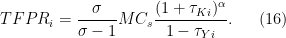
The first fraction, , is the markup charged over marginal cost by the firm. As the elasticity of substitution is assumed to be constant, this markup is identical for each firm, so generates no variation in . The second term,  , is the marginal cost of a bundle of inputs (capital and labor). The final fraction are the “wedges”.
  captures the additional cost (or subsidy if
  ) of a unit of capital to the firm relative to other firms.
  captures the revenue wedge (think of a sales tax or subsidy) for a firm relative to other firms. If either of those
  terms are not equal to zero, then will deviate from the efficient level.
* A note on multiple sectors * HK do this for all manufacturing sectors. That’s not a big change. Do what I said for each separate sector. Assume that each sector has a constant share of total expenditure (as in a Cobb-Douglas utility function). Then
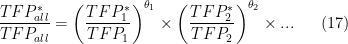
where  is the expenditure share of sector .

. Note that here the measurement does not have to take place using only past data. We could calculate the expected measured growth rate of GDP from 2015 to 2035 as
. Measured growth rate depends on the actual path (or expected actual path) of GDP.
) and the trend growth rate of the number of workers (which we’ll call
).

 is the measure of (labor-augmenting) productivity. What exactly does
  goes up, but what is that supposed to mean?
  ) and labor (
 ) are held constant?
 where
where  is intermediate goods. Productivity accounting could reveal to us a change in
  changes?
  . Innovation in logistics and inventory management makes the production function in 2014
  .
. 


 , and/or
 be
be  , so that
  is the price elasticity (in absolute value). As
  .
. total sectors. Each one produces with a function of
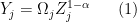
 is a given productivity term for the sector.
  is the factor input to production in sector
  , and units of
  , the “wage”, for each unit of
  ?
?
 , and now we really want to have concentrated productivity. I’m better off with one sector that is hyper-productive, while letting the rest dwindle. If I could, I would invest everything in raising productivity in one single sector. So a truly open economy that traded everything would want to load all of its R&D activity into one sector, make that as productive as possible, and just export that good to import everything else it wants.


 , and vary only in their value of
  .
.  and
and  technology, so
  . This makes some sense. If you have lots of some factor
  . But, if you use only that technology, then your
 ) in this setting is
 ) is rising, then so is output per worker. But wages will remain constant. This implies that labor’s share of output is falling, as
