NOTE: The Growth Economics Blog has moved sites. Click here to find this post at the new site.
This is a long post. It is partly in response to some questions from first-year grad students, and so it can be considered as notes for a lecture that might potentially be given to them at some point in the near future. For all that, it isn’t pitched at a high mathematical level. I think you could understand this without having ever done any kind of dynamic optimization work before.
Do savings matter for growth? This is an ill-formed question for several reasons. First, implicitly hiding in that question is the assumption that savings = investment. That doesn’t necessarily have to be true, and the events of the financial crisis in 2008 provide some evidence of this. So let us be more careful and say “Do investment rates matter for growth?”.
What do we mean by growth? You could really be referring to several things. “Do investment rates matter for the level of output per capita?” or “Does the investment rate today matter for the growth rate of output per capita today?” or “Does the investment rate – on average – matter for the trend growth rate of output per capita?”.
Let’s start with the simple cross-sectional relationship of investment rates and the level of GDP per capita. The following figure is from 2010, using Penn World Table 8.1 data. What you can see is that there is a (noisy) positive relationship between the two. Places with higher investment rates tend to be richer. If you used average investment rates over the last two decades or some other smoothing method, you’d get a similar picture. So we have some evidence that more investment is associated with a country being richer.

Hsieh and Klenow (2007), following others, noted that investment rates measured in PPP prices varied a lot more than investment rates measured in domestic prices. More simply, the share of domestic income that is spent on investment goods is similar across countries. However, the amount of real investment goods that this spending can buy tends to be very low in poor countries. This doesn’t mean that higher investment rates do not generate higher income per capita, it just means that there is a lot less variation in investment rates than we might think. This implies that the ability of differences in investment rates to explain cross-country differences in income per capita is limited. Hsieh and Klenow go on to show how it probably has more to do with differences in productivity in the investment good sector.

What about the effect of investment rates on growth rates, not the level of GDP per capita? Here we dip into the whole world of cross-country growth regressions. See Barro or Mankiw, Romer, Weil, or any of a few thousand papers from the 1990s. The simplest form is to regress the average growth rate of GDP per capita over some period (say 1960-2000) against initial GDP per capita (in 1960) and the investment rate (averaged over 1960-2000 as well). If you run this regression, then yes, you’ll get a positive coefficient on the investment rate. Places with higher investment rates grow faster – conditional on initial GDP per capita.
That conditional is crucial. Those regressions are not saying that higher investment rates raise the long-run growth rate of an economy. They are only saying that the level of GDP per capita will be higher along the balanced growth path of places with higher investment rates. The long-run growth rate along that balanced growth path is probably similar across all those countries. If you remember the post I did about convergence and the analogy with people driving down the highway, these regressions tell us that investment rates allow you to move farther up the line of cars, but ultimately you still have to settle in behind the sheriff and go 65.
Why is there a relationship of investment rates and growth? The “Duh” answer to this is that capital matters for producing output. More investment, more capital, more output. What we really want to ask if “Can we describe the dynamics of investment and growth?”.
The workhorse model for these dynamics is often called the Neo-classical growth model. It is often the first dynamic model you learn in graduate school, and it sits at the heart of all your favorite (or despised) DSGE models. The Neo-classical growth model goes by a lot of names. I tend to call it the Ramsey model, and will do so throughout this post. It’s also sometimes referred to as the Cass-Ramsey-Koopmans model, or more bluntly as the Solow-model-with-endogenous-savings.
The Ramsey model is a model of investment and growth. It is not a model of the effect of investment on growth. The effect of investment on growth is baked into the Ramsey (and the Solow, for that matter) by the accumulation equation for capital
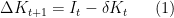
and the assumption that output depends on capital,  . If you raise
  , then you accumulate more capital, and if you accumulate more capital output goes up. This is purely mechanical.
In the Solow model, is s fixed fraction of output. In the Ramsey model, the choice of how much of output to invest – how big will be – is determined by a forward-looking optimization problem, typically with a representative agent. Hence investment and growth are jointly determined in the Ramsey model, and both are dictated by the current state of the economy, which is captured by the current capital stock, .
Does the Ramsey provide a good description of the world? More precisely, does it provide a good description of how investment rates are related to GDP per capita or the growth of GDP per capita?
For explaining the cross-country relationship of investment and levels of output per capita, the Ramsey model is no better than the Solow model. The Solow says that countries with higher exogenous investment rates (typically denoted  ) will be richer. The Ramsey says that countries with higher exogenous patience preference parameters (typically denoted
  or
or  ) will be richer. This a distinction without a difference. The Solow might be superior here, in that it leaves open any possible reason for investment rates to differ, while the Ramsey forces you into thinking about patience parameters.
For explaining the time-series relationship of investment and output per capita, or investment and growth, the Ramsey model can actually offer us something. The Solow model’s fixed investment rate is just that, and hence there is no way (aside from a series of remarkable exogenous coincidences) that the investment rate will change as a country becomes richer or poorer. In contrast, the Ramsey model’s whole raison d’etre is to describe how investment rates change as output per worker changes.
What does the Ramsey model predict? That depends on the specific parameter values you choose. You can get the Ramsey model to predict investment rates that rise with output per capita or fall with output per capita if you tweak things just right. If you try to discipline the parameters in the typical way done in macro – a capital share of about 0.3-0.4, an inter-temporal elasticity of substitution of about 1/3 – then you get that savings should fall as output per worker rises. In other words, when a country is below its balanced growth path, it is predicted to save a big fraction of output, and this fraction is predicted to decline as it approaches it’s balanced growth path. Basically, the “high” elasticity of substitution means people are willing to invest a lot today (i.e. consume little) in return for lower investment rates in the future (i.e. high consumption). A country below its balanced growth path that invests a lot will grow quickly, and hence the Ramsey predicts that investment rates and growth rates should track each other.
Does this prediction hold up? In some cases, it looks great. Here’s a plot of the investment rate in Germany after WWII until now, along with the plot of the forward-looking 10-year average growth rate of output per capita. This looks qualitatively like exactly what the Ramsey model predicts.

So everything is great, right? Not quite. There are a number of other examples where the pattern actually looks nothing like what the Ramsey predicts. Here’s a plot from Japan, and from 1950 to 1980 this works exactly opposite of what the Ramsey says, but perhaps from 1980 forward it works?

Or consider Korea, where the spike in growth rates precedes the spike in investment rates, and then once growth starts to slow down after 1980 as Korea approaches the balanced growth path, the investment rate stays level. Or India, where there’s been a spike in investment rates recently, well after growth started to accelerate.


This doesn’t necessarily mean the Ramsey is wrong, but to explain these patterns we need to start delving into remarkable exogenous coincidences again. Productivity shocks that happen at just the right time, or unexplained shifts in patience parameters at exactly the right moment.
There’s another issue, though, which is that even the Germany figure doesn’t match the prediction of the Ramsey model. Under the typical parameters, the Ramsey says that both investment and the growth rate should have declined much faster than they actually did. Another way of saying this is that convergence speeds are predicted to be incredibly high in the Ramsey model. For Germany, given the starting point in 1950, the growth rate should have already dropped to about 2.5% and the investment rate to 20% by about 1965.
I’ve mentioned before that empirically, the convergence rate is about 2% per year, meaning that 2% of the gap between actual GDP and the balanced growth path closes each year. We find that estimate coming out of all sorts of settings. The Ramsey model predicts convergence rates of up to 30-40% for countries like Germany in 1950. It’s not even in the realm of empirically plausible.
A more thorough examination of the correlation between investment rates and growth can be found in Attanasio, Picci, and Scorcu (2000) paper, which builds on Carroll and Weil (1994). Both find that, if anything, higher investment rates Granger-cause lower growth rates. They also find that higher growth rates Granger-cause higher investment rates. In other words, a shock to growth is likely to be followed by higher investment rates in the future – which is backwards from what we baked into the Ramsey model. Second, shocks to investment rates are actually likely to be followed by lower growth rates – for this you could perhaps argue as demonstrating that higher investment causes convergence, and hence the growth rate would fall. But it is hard to reconcile with what we’d expect to see in the Ramsey model.
So….What exactly is the Ramsey model good for? Off the shelf, the Ramsey is a poor descriptor of the time-series evidence, and is needlessly complex for explaining cross-sectional relationships. But in failing, you can understand what might need to be added to match the time-series data.
To “slow down” the convergence speed in the Ramsey model, for instance, you can drop the assumption that all capital is perfectly substitutable across firms. I did this with Sebnem Kalemli-Ozcan and Indrit Hoxha, and once you lower the elasticity of substitution to 3 or 4, then predicted convergence speeds in the Ramsey become reasonable.
To match the Granger-causation of growth to investment rates, you can break the assumption that preferences are time-separable. This is what Carroll, Overland, and Weil (2000) do by adding habit formation into the Ramsey. Basically, your marginal utility depends on how much you consume today and how much you consumed yesterday. Because of this, your response to shocks is relatively slow, and so when growth ramps up (due to a productivity shock, for example) the savings rate doesn’t instantly jump up, but takes a while to respond.
To capture the time-series experiences of places like India or Japan you could appeal to some kind of exogenous coincidence. Just because they are implausible doesn’t mean they can’t occur. S*** happens, and so the Ramsey could be totally right, just masked by a series of crazy shocks to productivity, preferences, institutions, etc.. The take-away from this could be that you should stop worrying about trying to explain growth as something that has a common process in all places, and focus on explaining the growth of a specific place in detail.
You can also remember that the aggregate data we are looking at is exactly that, aggregate. Which means that it is the summation over millions of little individual decisions, and so the representative agent in the Ramsey model is probably not a good approximation. But saying that you should allow for heterogeneity in the model is a lot like saying that you should study each country individually, as the heterogeneity is going to be unique.


![\displaystyle Growth = \frac{y_{t+1}-y_t}{y_t} = (1+g)\left[\lambda \frac{y^{\ast}_t}{y_t} + (1-\lambda)\right] - 1. \ \ \ \ \ (1)](https://s0.wp.com/latex.php?latex=%5Cdisplaystyle++Growth+%3D+%5Cfrac%7By_%7Bt%2B1%7D-y_t%7D%7By_t%7D+%3D+%281%2Bg%29%5Cleft%5B%5Clambda+%5Cfrac%7By%5E%7B%5Cast%7D_t%7D%7By_t%7D+%2B+%281-%5Clambda%29%5Cright%5D+-+1.+%5C+%5C+%5C+%5C+%5C+%281%29&bg=ffffff&fg=000000&s=0&c=20201002)


 is the “tax rate”, and this tax rate is meant to capture both formal taxation and any other frictions that limit profits (e.g. regulations).
  is the markup that the owner can charge over marginal cost for their idea.
  is therefore the difference between price and marginal cost. The more indispensable your idea, the higher the markup you can charge. For instance, there are big markups on many heart medications because your demand for them is pretty inelastic. The markup on a new type of LCD TV is very low because there are lots and lots of almost identical substitutes.
  is the marginal cost, which here we can think of as the wage rate you pay to run the business that produces the good or service based on your idea.
  is the number of “units” of the idea that you sell (pills or TVs or whatever). Together,
  represents “market size”. If the wage rate or quantity purchased go up, then your absolute profits rise. The effect of
  goes up should generate more ideas. My issue with Michael Strain’s article, and others like it, is that when they think of “progressive social policy”, they think only of the cost
 – is going to be governed by something like the following process
 is a function that describes how many resources we put towards innovation, like how much time is spent doing R&D, or how much is spent on labs. That allocation depends on profits,
  . Social policies can not only raise
  , is a term that captures the effect of the level of innovation,
  , on the growth rate,
  , and this means that the growth rate will end up pinned down in the long run, and social policies will have a positive level effect on innovation. If you are of the opinion that
  , then policies have permanent effects on the growth rate. It isn’t important for my purposes which of those is right.
 , is just
 . We might imagine that
  . You calculate it as
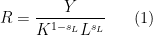
 is GDP,
  is the capital stock, and
  is the labor supply (which you could measure in units of human capital if you wanted). The term
  is labor’s measured share in total output.
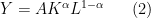
 , not
, not  are “true” technological coefficients. The measure how GDP responds to stocks of capital and labor. But we don’t know them. All we know is
  is the left-over amount of GDP paid out as returns to capital and profits.
  . And under a very precise set of conditions, these two things would be equal. If we had competition in output markets, and competition in factor markets, then
 is the mark-up of price over its marginal cost. For example, if
  , then the price charged is twice the marginal cost of production (which is the cost of hiring labor and capital). Under competition, P=MC, so
  , and
, and 
 .
. 
 as the growth rate of the capital/labor ratio,
  . Again, if we had perfect competition and
  , would be exactly equal to the growth rate of “true” productivity,
  . But once
  ? That came from assuming that firms are cost-minimizing (not necessarily profit-maximizing even, just cost-minimizing). That cost-minimization problem also implies that the following has to be true
 is the share of GDP that gets paid out as profits – A/K/A rents. What this relationship says is that if the share of output going to rents rises, then so must the markup. Or think about it the other way. If firms can charge higher markups, they must be earning more in rents/profits. This is just a mechanical relationship, so it doesn’t necessarily have to be driven by one or the other.
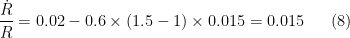
  over the last 30 years. Let the true growth rate of innovation be
  over the entire last 30 years (yes, an assumption). Start out 30 years ago by assuming the labor share is
  and that the markup is
  , so firms charge 10% over marginal cost. This means that measured productivity growth is
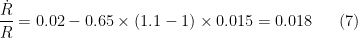
 , and let the markup rise to
  . This is a pretty big markup, but for the moment I’m just trying to establish a point, so bear with me. We get that measured productivity growth is